Statistical Learning Theory

Stats Learning Theory Course Slides Notes

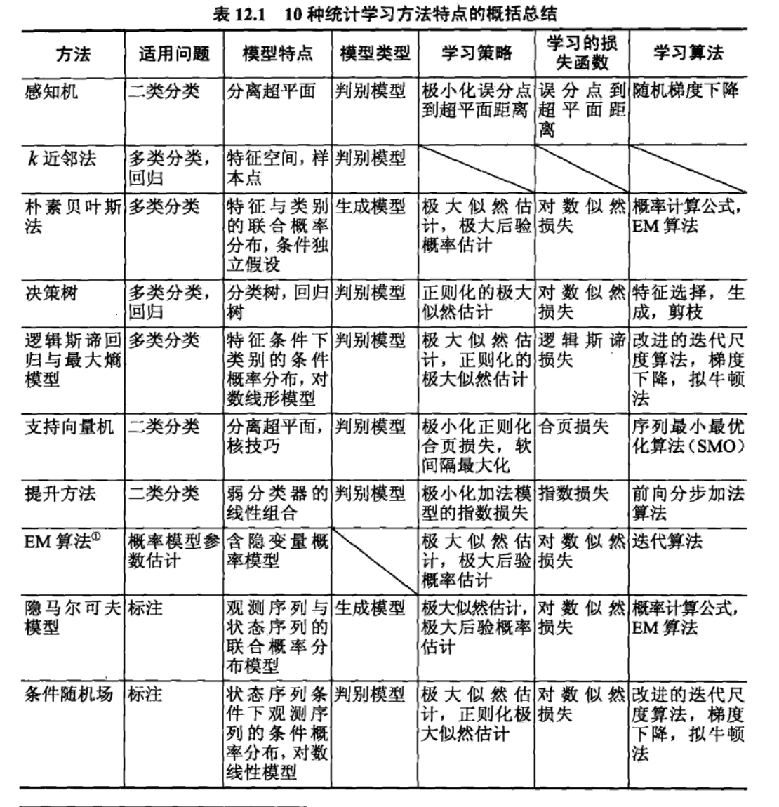
1. risk theory

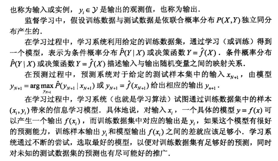
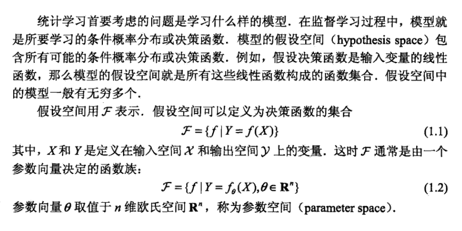
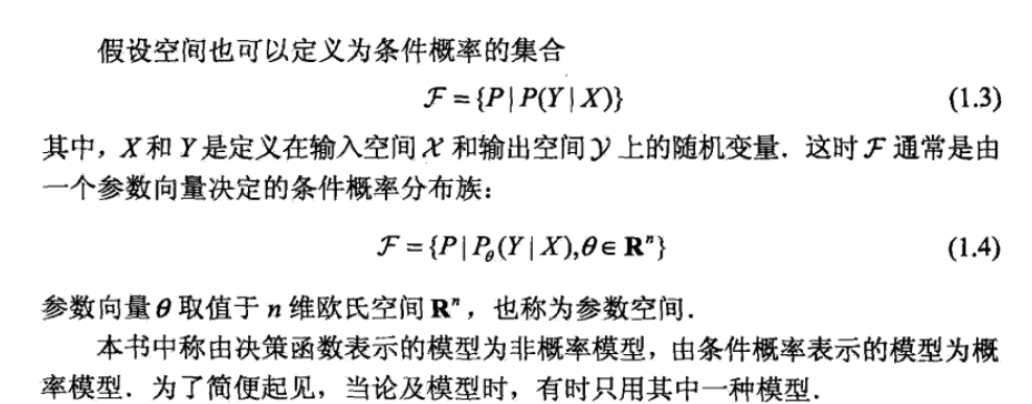
1.1. learning algorithm & loss functions (1-1, 3-1)

f -> h, L -> R

• Def: learning algorithm Ln (3-1)

  Usage: from data to algorithms space

  

  • Def: weakly consistent / strongly consistent （3-1)

    

    Note: \(\hat{h_n}\) is random variable since it completely depends on iid data when \(L_n\) is fixed. (3-1)

    

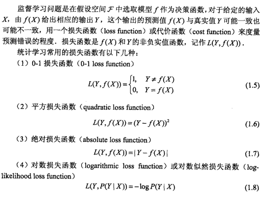
• Def: loss (loss function) (1-1)

  

  Example: the relation of max likelihood & loss function (1-10)

  

  Example: (1-10)

  

1.2. loss functions

1.2.1. E-f-loss (1-1, 3-1)

Goal: we analyze what decide a good f function and what are the bounds between f and f star.

• Def: E-f-loss (generalized expected risk) (1-1)

  

  (3-1)

  

• Def: min-E-f-loss (minimal generalized expected risk) (1-1)

  

  • Theorm: min-E-f-loss for binary classification is bayes classification

    (1-1)

    

    (3-2)

    

    

    Proof: (3-2)

    

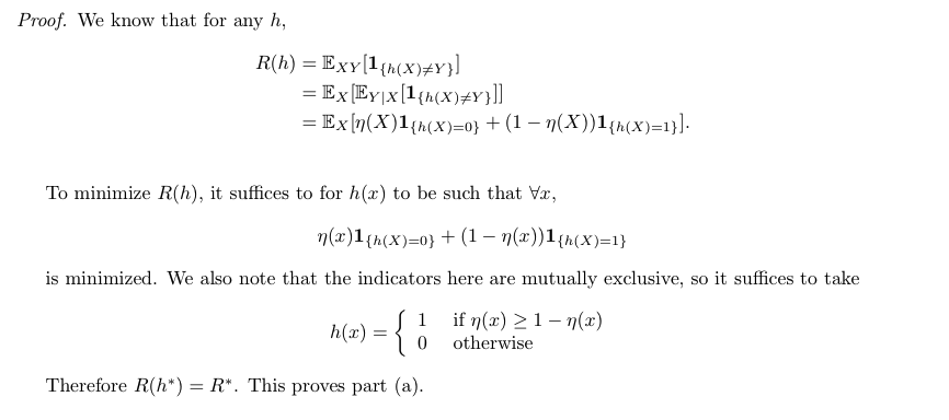
• Theorem: min-E-f-loss for binary classification(3-2)

  

  Proof: (3-2)

  

  Note:

  

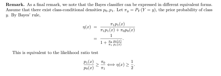
• Def: other form of bayes (3-2)

  

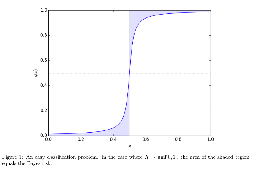
  Note: figure of bayes risk (from 3-2)

  

• Theorm: E-f-loss - min-E-f-loss (1-1, 3-1)

  Usage: find f to estimate f*

  (3-2)

  

  Proof:(3-2)

  

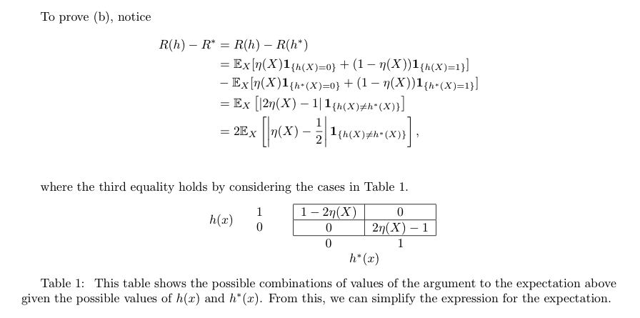
  Note:(3-2)

  

  (1-1)

  

  Proof: (1-1)

  

1.2.2. E-$f_ $-loss (plug-in classifiers) (1-1, 3-2)

Goal: we analyze the usage of plug-in classifiers.

• Def: Plug-in classifier: swe can see that \(\eta\) is what we what to estimate, the goal turns to find a better \(\eta\). (1-1)

  

  (3-2)

  

• Theorem: E-\(f_\hat{\eta}\)-loss - min-E-f-loss (1-1)

  Usage: when using \(\hat{\eta}\) to find best f, instead of directly finding f, what's the bound?

  (1-1)

  

  Proof: (1-1)

  

  Note: figure / pros & cons to use \(\hat{\eta}\) to minimize E loss (1-1)

  

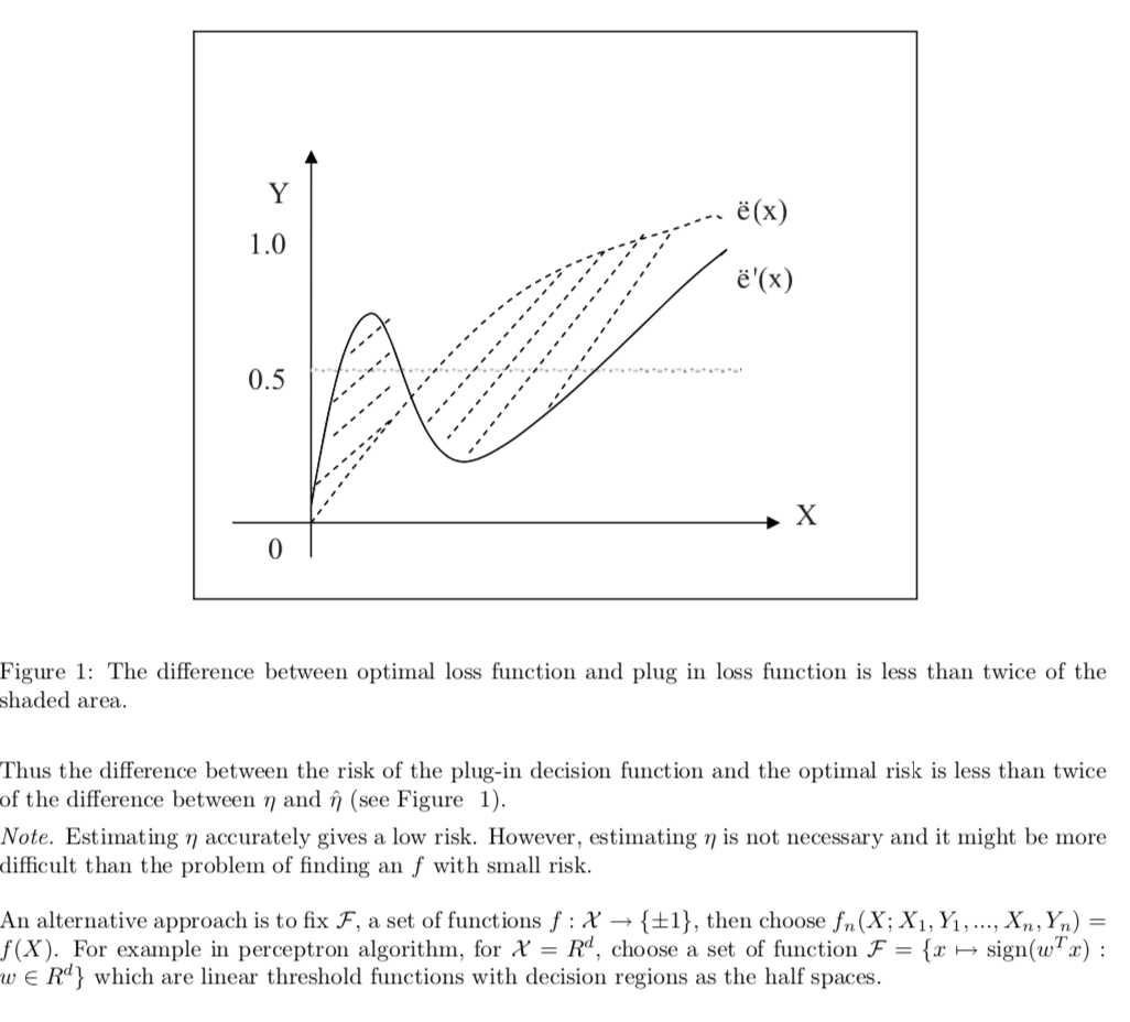
  (3-2)

  

  Note: (3-2)

  

1.2.3. E-f-newloss (1-6, 1-7)

Goal: we analyze usage of different loss functions.

• Def: E-f-newloss

  

  Note: SVM

  

• Qua: => elaboration

  Usage: we can minimize E-f-newloss by minimizing the follows at every x/

  

• Def: new elements to compute min-E-f-newloss, \(H(\eta)\) means the lowest point of all f, all x.

  

  Note: SVM

  

  

• Qua: when \(\phi\) is convex => \(H ^{-}(\eta) =\phi(0)\)

  

• Def: classification - calibrated

  

  Example:

  

  • Qua: necc & suff

    Proof: too long

  • Qua: real gap is bounded by E-f-newcalibratedloss

    

    Proof: too long

    Example: in the case of SVM, \(\phi\) is a given convex function, therefore we can conpute \(H(\phi)\) and yield a upper bound for the real gap. which means when training performs good, the result will most likely be the same.

    

    Example: adaboost is the same, \(\phi(a)\) is convex and we can again use theorem 2.2

    

    Example: adaboost(1-13), a more detailed explaination, \(\phi\) is class-calibrated, so we can use theorem 2.2.

    

    

1.2.4. Em-f-loss (1-2,13, 3-3,4,5)

• Def: Em-f-loss

  (3-3)

  

  (3-4) the best Em-f-loss h

  

  Note: (3-3)

  

• Qua: Em-f-loss converge to E-f-loss (1-13)

  

  Proof: why E(empirical risk) = generalized : E(h) is actually P(y|x), so $E((h))=_n E(1(...))/n=_n p/n = p $

  

  Note: (1-13)

  

1.2.4.1. empirical bounds (3-3,4,5)

Goal: In this chapter we'll discover the bounds for empirical loss, or in other words, how well can we train the algorithm if we use empirical algorithms?

This is the whole picture: that we use em-loss to estimate the loss function.During this section, we'll use different tools to bound between \(\hat{E}\) and E, such as VC & hoeffding bound, etc. (1-18)

1.2.4.1.1. uniform deviation bound

Goal: if we have bound generated by EPT, we have a goal proved.

• Theorm:: => Em-f-loss - E-f-loss, uniform deviation bound (bound the performance of em)(not know h)(3-4)

  

  Proof: (3-4)

  

  note:

  

• Theorm: => E-fem-loss bound case 2 unifrom devia bound (3-4)

  

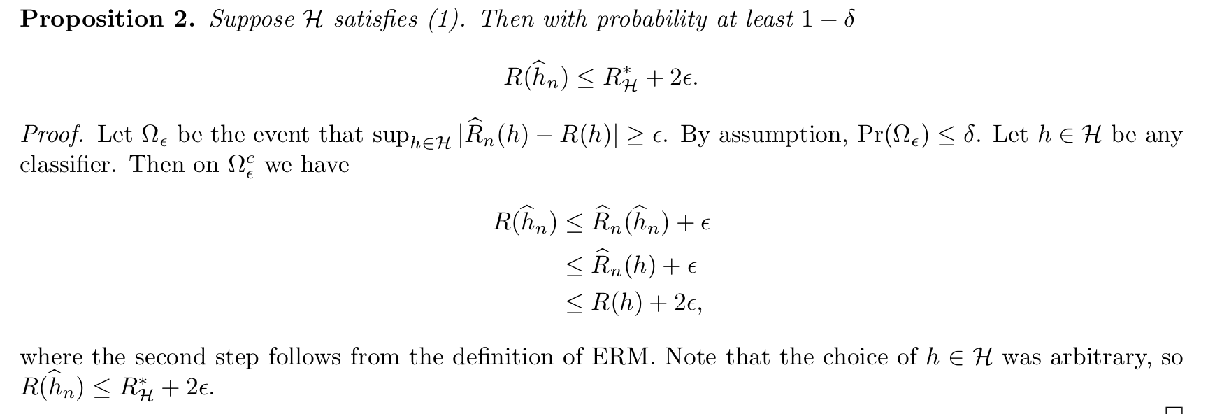
  Note:(3-4)

  

• Theorm: => E-fem-loss probability bound2 (3-4)

  

• Theorem => Em-f-loss bound 3, if zero error case (3-4)

  

1.2.4.1.2. vc bound

the bound of EPT generated by vc

• Theorm:: => Em-f-loss vc bound 4 (3-5)

  

  Note: that the right side can be bounded

  

  • Corollary:

    

    Proof: follows from theorem using an argument like that when \(|H|< \infty\)

  • Corollary: this is obvious from theorem.

    

• Theorm: => learnable (3-5)

  

1.2.4.1.3. bound improvement by approximation error

1.2.4.1.3.1. UAP & approximate error

• Intro: decomposition to est ( discussed in above, basically random) + app ( not discussed before, decide by algorithm pool H). In this lecture we'll talk about app error (3-6)

  

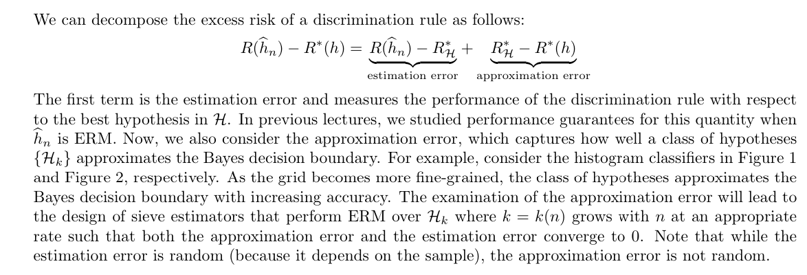
  Def: universal approximation property (3-6)

  Usage: UAP is when H pool grows, the approximation error converge to 0.

  

  Note:(3-6)

  

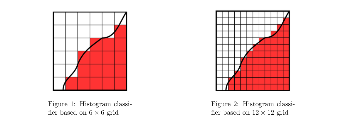
• Theorem: special Hk consist of piecewise constant classifiers => (3-6)

  

  Example:(3-6)

  

  

1.2.4.1.3.2. sieve estimators

• Def: best estimate classifier from H (3-6)

  

• Intro & Def:Strong Universally Consistent, why and what is a sieve estimator, basically to let the whole thing go to 0 simutaniously. (3-6)

  

• Theorem: UAP & k(n) sequence => (3-6)

  Proof: (3-6)

  

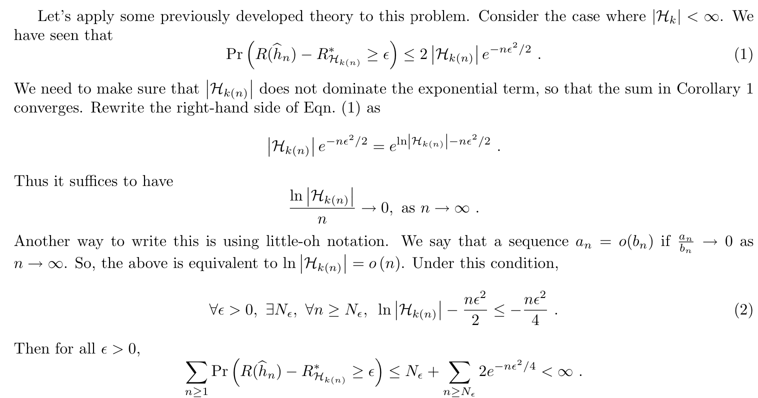
  • Corollary: similar to theorem => (3-6)

    

    Note: (3-6)

    

• Theorem: UAP + VC bound => (3-6)

  

  Proof:(3-6)

  

1.2.4.1.3.3. rate of convergence

• Def: rate of convergence(3-6)

• Theorem:(3-6)

  Note:(3-6)

  

  Example: box-counting class (3-6)

1.2.4.1.4. Rademacher averages bound (1-18)

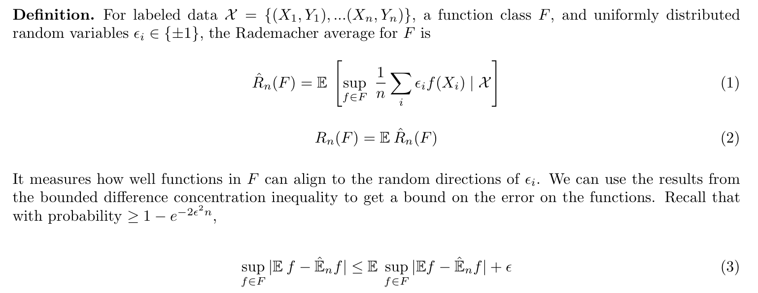
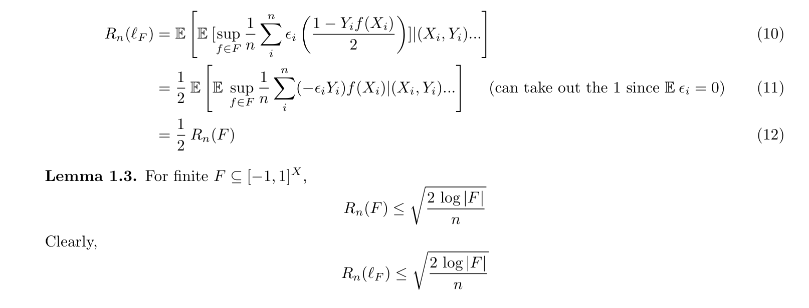
• Def: RA

  Usage: how well function class F align to random directions, as well as to provide a upper bound

  

  • Qua:

    

  • Qua:

    

    Note:

    

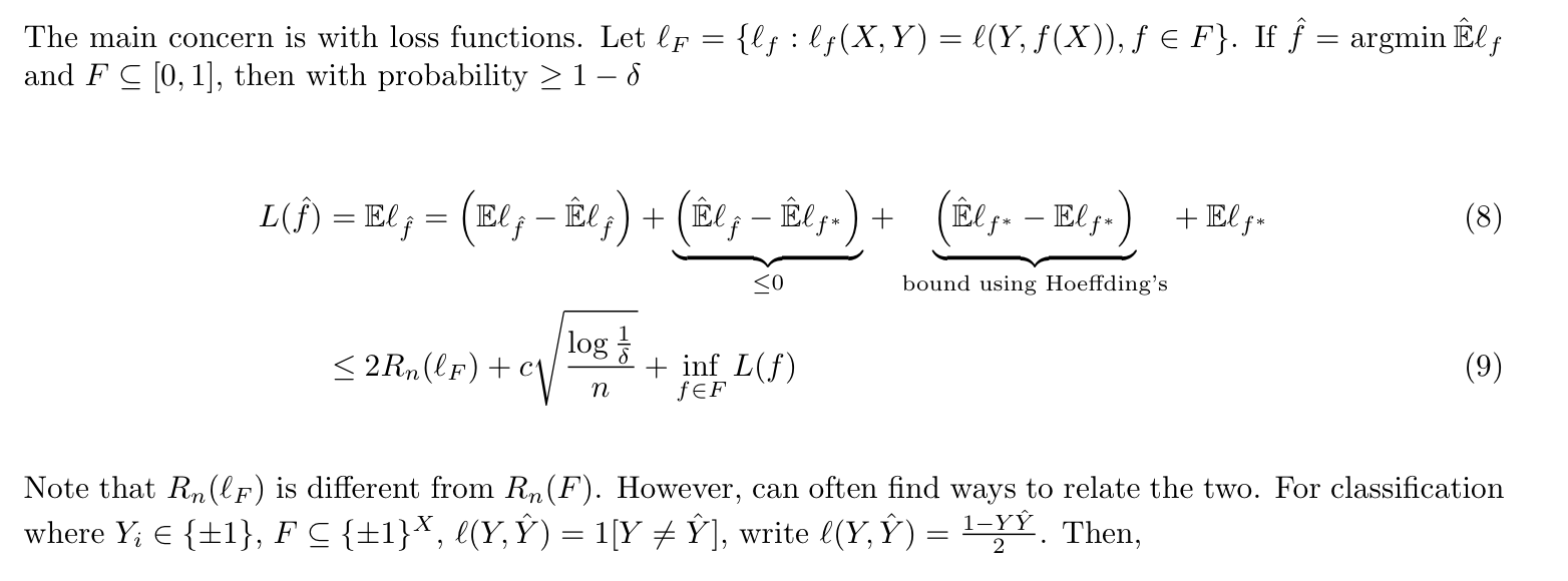
  • Note: concern with loss function

    

    

1.2.4.2. empirical processing theory

Goal: to make Em & E close enough, Empirical Process theory allows us to prove uniform convergence laws of various kinds. One of the ways to start Empirical Process theory is from the Glivenko-Cantelli theorem. This leads to the question of whether the same idea can be generalized to other function classes.

1.2.4.2.1. Glivenko-Cantelli

This is where we'll start, by proving GC and go further, GC means that for certain class of mapping G, we have the following: and in the chapter after we'll generlize G .

1.2.4.2.1.1. empirical distribution function (book, 2-2)

• Def: empirical distribution function

  Usage: is a statistic

  (book)

  

  (2-2)

  

• Qua: => range (book)

  

• Qua: => other interpretation(book)

  

• Qua: => limits (book)

  

  (2-2)

  

1.2.4.2.1.2. GC class & theory (1-16, 2-2)

• Def: GC class (1-16)

  Usage: difference between P-GC is the supPn.

  

• Theorem: GC theory

  (1-16)

  

  (1-17)

  

  Note: this is equivalent(1-17)

  

  (2-2)

  

  (book)

  

  Note: Fn and F is very close when n is large

  

1.2.4.2.2. generalized Glivenko-Cantelli (1-13,14, 2-6)

1.2.4.2.2.1. symmetrization lemma (2-5)

Lemma in this section is important to generalize GC.

• Def : recall distribution function (2-5)

  

• Def: Rademacher variables (2-5)

  

• Lemma: => first symmtry bound the Fn-F(t) (2-5)

  

  Usage: using two indenpendent stochastic process to set upper bound for one .

  Example: (2-5)

  

• Lemma: second symmtry => aallowsustoreplacethedifferenceFn−Fn′ withasingleempiricalquantity consisting of n observations. We can further bound the latter so that the bound is independent of the data ξ. (2-5)

  

  Usage：using independent variables to set upper bound for GC (2-5)

  

  Proof: (2-5)

  

1.2.4.2.2.2. generalized GC

Using Lemma above to prove GC

Goal: for every F, make Em & E close enough. we can first generalize the Glivenko-Cantelli theorem (a special F space).

• Intro: what is and why we should use uniform convergence: (1-13, 1-14)

  if there's only one function in F, we simply use law of large numbers, then we can prove convergence, but it is of no use.

  

  Example: when F contains more functions and here the case is when dataset are separated, empirical risk are sometimes not convergence to real risk. (1-13)

  

  Example: the GC theorem in function way (2-6)

  

• Intro: using Lemma1 in 1.2.3.2.3 to empirical functions (2-6)

  

  Usage: when we F specialize to indicators (2-6)

  

  

​

1.2.4.2.3. vc class and stuff

Vc & covering number are powerful tools to empirical learning.

######vc class (2-6,7, 3-5)

• Def: vc class

  Usage: vc class , C is a collection of sets，X is the largest set, Vc is：given n points from X, if subsets of C cannot separate X into \(2 ^{n}\) parts，then \(V ^{C}=n\), mind that we should go from n =1 to above, and see if we could find the x points that could be shattered by this set, if not we shop and set Vc = n. So basically, the larger Vc, the better C is in regards to shatting set X.

  (2-6)

  

  Example: $V ^{C} = 2 $ since given \(x1=1, x2=2\), you can't separate them. (2-6)

  

  Example: half space (2-7)

  

  Example: subgraph (2-7)

  

  (3-5), nth shatter coeffcient is m(n), for all n < Vc, we say F/H shatters {x1...xn}

  

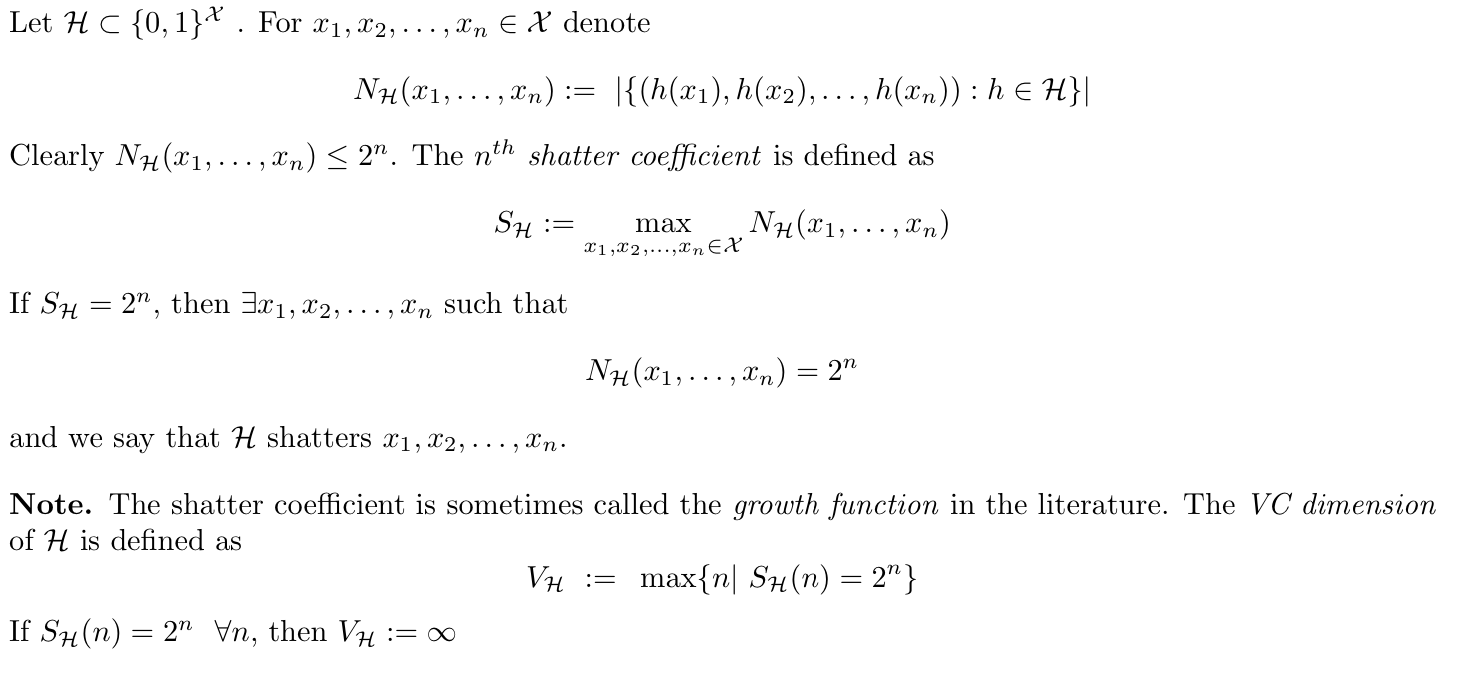
  Example: (3-5)

  

  

  

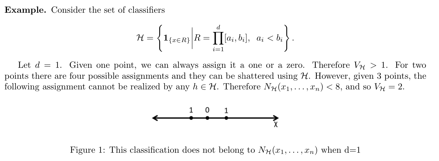
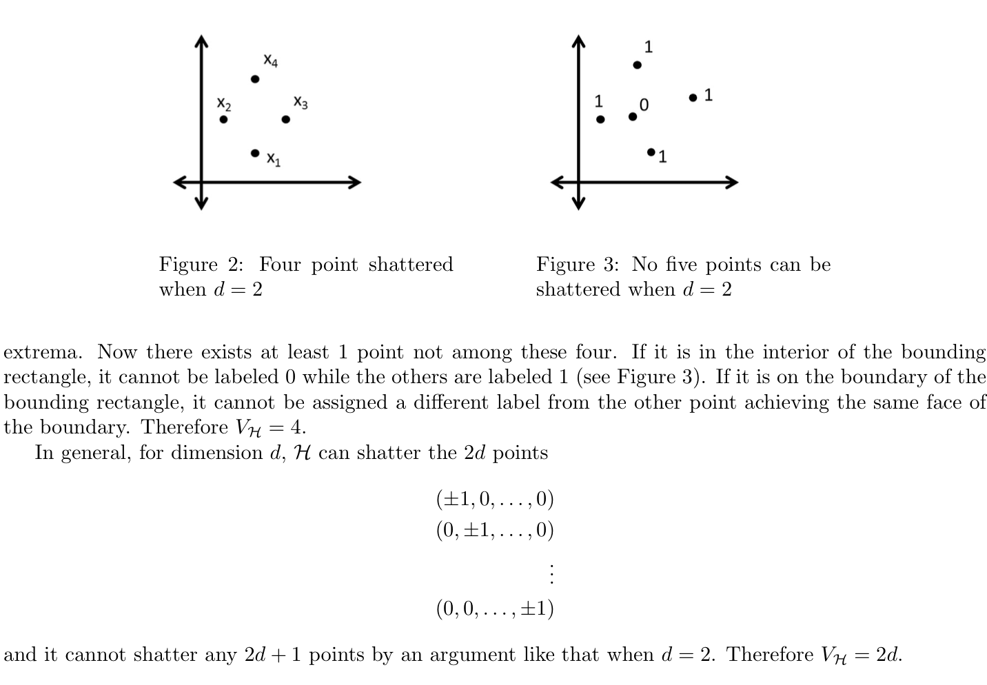
  Example: (3-5)

  

  Example: (3-5)

  

  

• Lemma: => bound Vc for a broad family of classes

  

• Lemma: => Sauer's the relation ship between m(n) and Vc

  (3-5)

  

  (2-6)

  

  Proof: (2-6)

  

  Note: that we can use VC to see Pn, use m(n) to indicate the \(2 ^{n}\) subsets of all, and we use lemma to get a upper bound of Pn0 (2-6)

  

  

  • Corollary: (3-5)

    

    • Corollary: (3-5)

      

    • Corollary: (3-5)

      

• Qua: operation (2-7)

  

  ​

1.2.4.2.3.1. covering number (2-7, 2-8)

• Def: covering number (a more powerful way than VC) (2-7)

  Usage: a covering number is the smallest number of functions that can approximate any f with metric Q in F. Apparently larger N1, the more complex class F, the more powerful it is in regards to classification. Here N1 means F is constrained within \(L ^{1}(Q)\)

  

  Note: not unique s (2-7)

  

• Theorem: => apporximation lemma, giving an upper bound for covering number of VC dimension(2-8)

  

  Usage: (2-8)

  

1.2.4.2.3.2. entropy

• Def: metric entropy (2-7)

  Usage: metric entropy is log N1.

  

  Example: (2-7)

  

  Proof: computing cover number for F. Using definition of covering number, constructing \(\hat{f}\) for F (2-7)

  

  

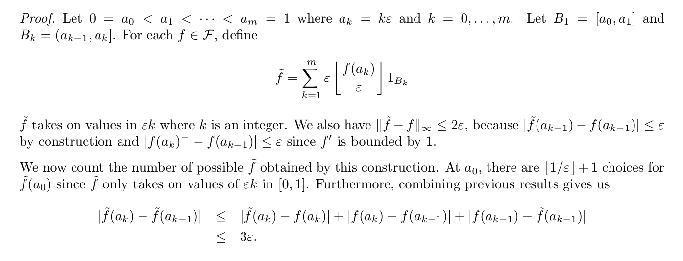
• Def: totally bounded (2-7)

  

• Def: entropy with bracking (2-7)

  Usage: Np,B means the smallest of m pairs of functions that can approximate any f in F.

  

• Qua: relation of metric & brackeing entropy (2-7)

  

1.2.4.2.3.3. vc theory for sets(3-5)

• Theorm: VC theory => convergence guarantees for an empirical risk minimizing classifier when the VC dimen- sion of the classifier set H was finite. (3-5)

  

  • Corollary DKW

    

• Qua: operation.

  

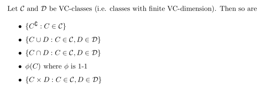
1.2.4.2.3.4. mono layer (a special classifier)(3-5)

• Def: see page 8 of class_3 lecture 5

  • Theorm: => bound of expected shatter coefficient

    

    • Corollary: => convergence

      

1.2.4.2.4. P-Glivenko-Cantelli (for class F)

This is where we finally arrived at, the generalized GC.

• Def: P-Glivenko-Cantelli class(2-8)

  

• Def: envelop (2-8)

  

  • Theorem: => P-GC (2-8)

    

    Note: intuition for condition of metric entropy (2-8)

    

    Proof: way too long

    Example: (2-8)

    

1.3. alternative loss functions

1.3.1. maximum likelihood

• Def: maximum likelihood \(l(f(x_i),y_i)\)

  Usage: turn to an alternative minimization goal, only available when the output is conditional probability

  

1.3.2. probably approximately correct (1-13, 3-4)

• Def: PAC (1-13)

  Usage: turn to an alternative goal.

  

  

  

  ​

  • Def: probability approximate corret condition (1-13)

    

    

• Qua: PAC insights (1-13)

  

• Def: PAC learnable (1-13)

  

• Def: PAC definition 2 ( 3-4)

  

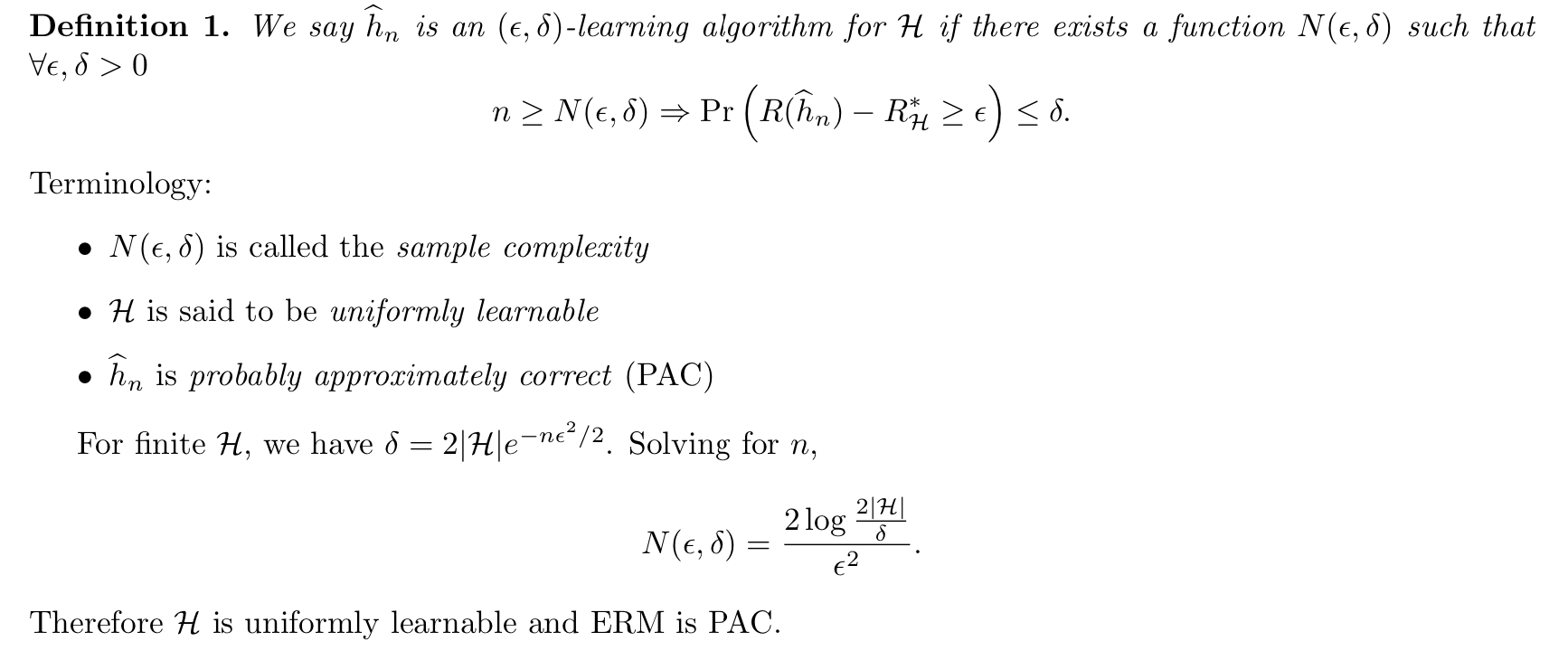
2. supervised algorithms

2.1. decision theory

• Def:

  

  

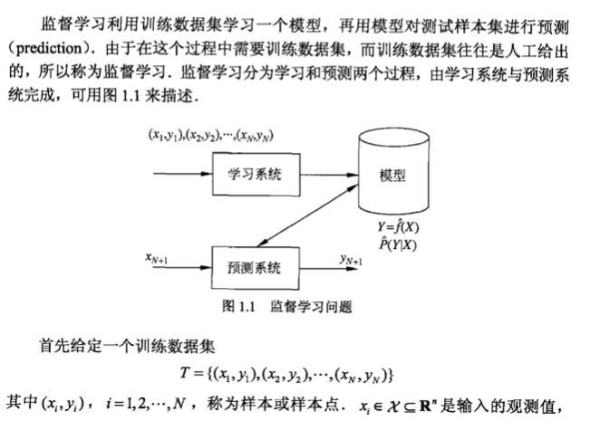
• Note: model choosing -> loss function choosing -> optimization (training) -> validation

2.1.1. model

• Def: model

  

  

2.1.1.1. generative model

• Def:

  

  • Qua:

    

2.1.1.2. discriminative model

• Def:

  

  • Qua:

    

2.1.2. loss function

• Def: loss function

  

2.1.2.1. E f loss

• Def: E f loss function

  

  • Note: goal of training is to make this small

2.1.2.2. Em f loss

• Def: Em f loss

  

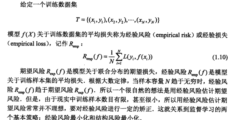
  • Note: E f loss can't be obtained

• Def: regularization

  

  

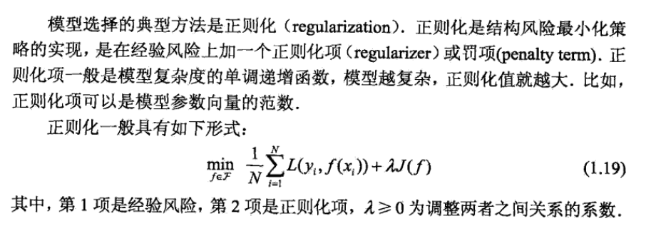
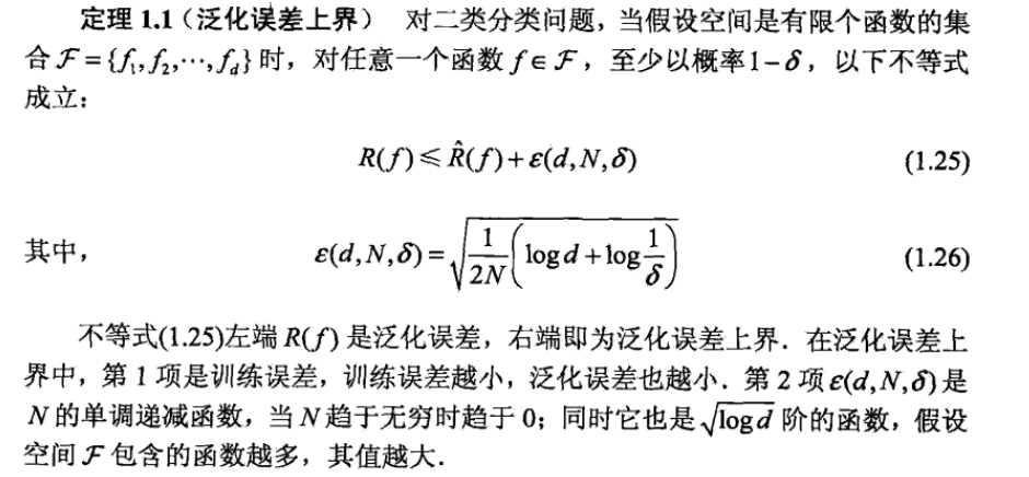
• Def: Em-f*-loss

  

  • Theorem: upper bound

    

2.1.2.3. max likelihood

• Def: max likelihood

2.1.3. optimization algorithm

• Def:

  

  

2.1.4. validation criteria

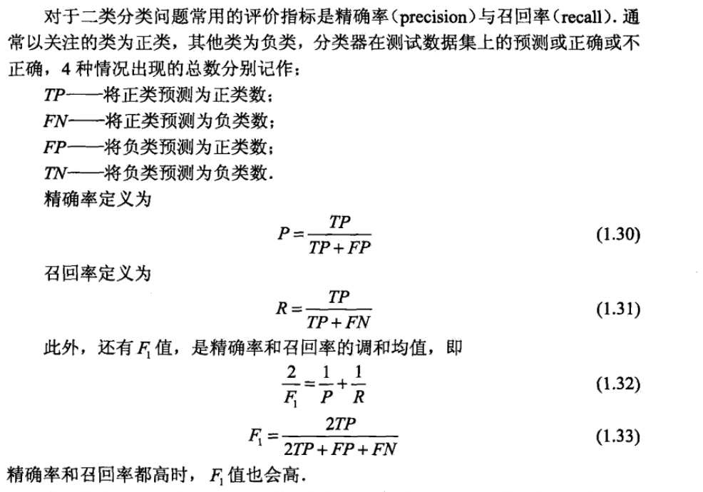
####TN & TP

• Usage: criteria for 2-classification

• Def:

  

• Def

  

  

2.1.4.1. accuracy

• Usage: classification for > 2

• Def;

  

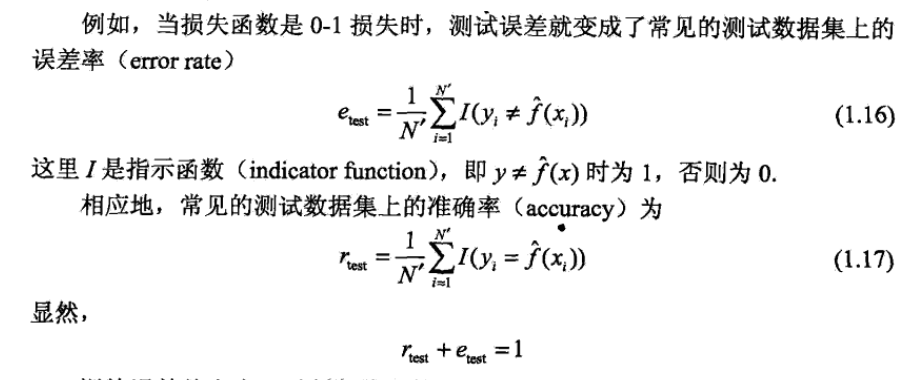
2.1.5. validation improvement

2.1.5.1. validation set

• Def:

  

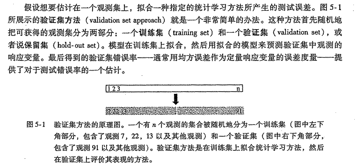
  • Qua: cons

    

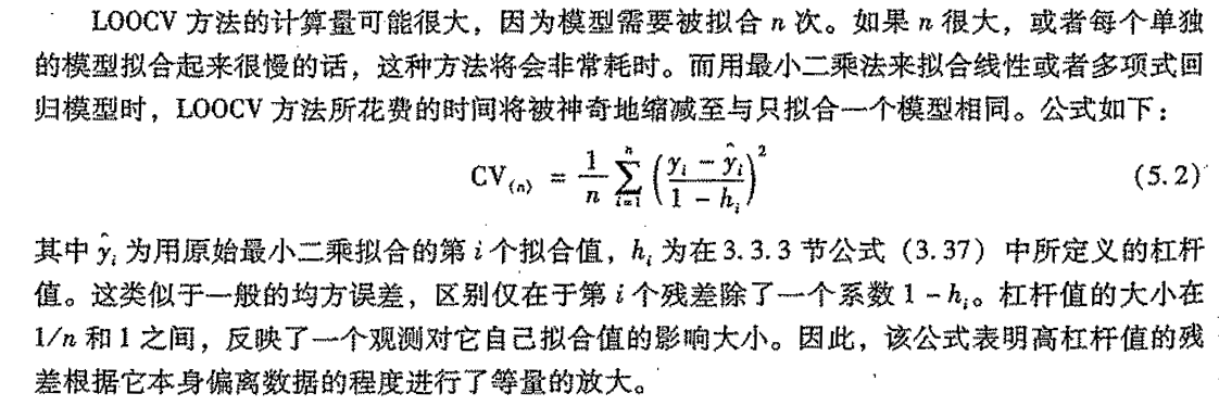
2.1.5.2. leave one out validation

• Def:

  

  • Qua: pro

    

    

  • Qua: special for regression

    

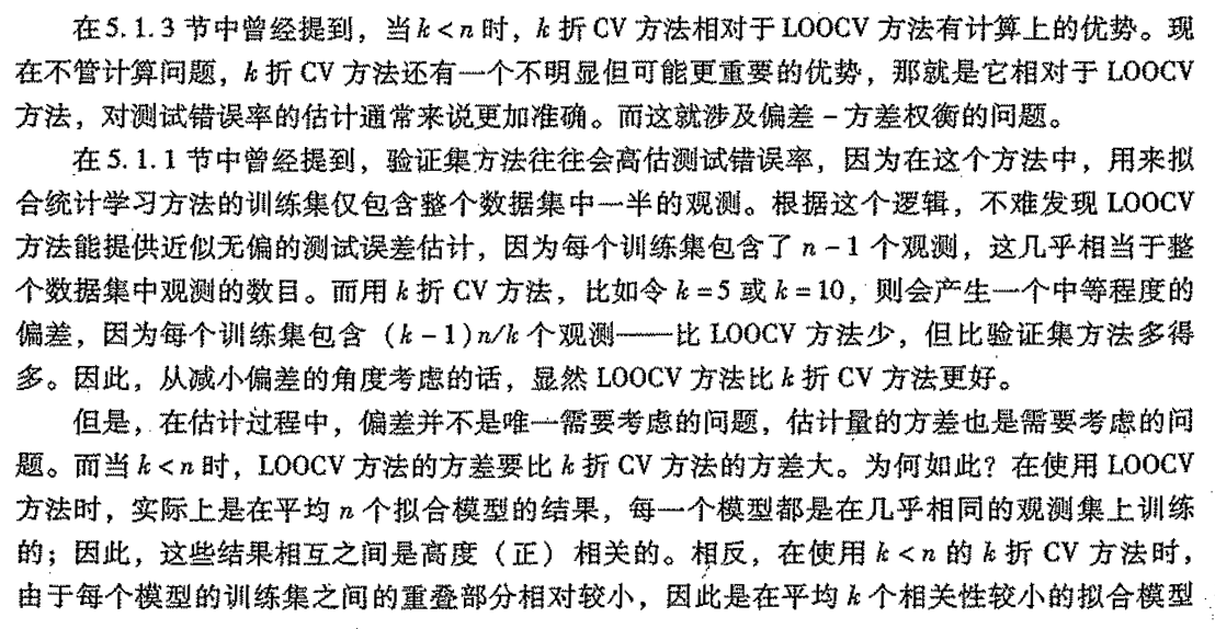
2.1.5.3. leave k out validation

• Def:

  

  • Qua: balance

    

    

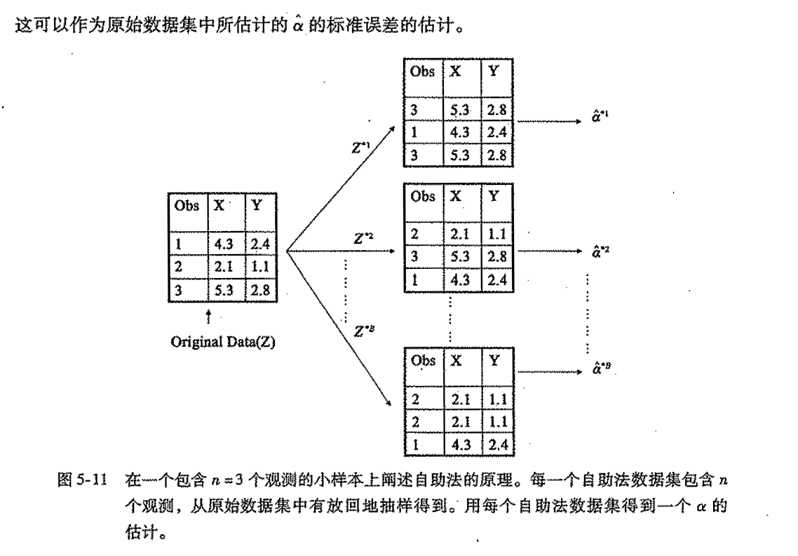
2.1.5.4. bootstrap

• Def:

  

  

2.1.6. high dimension problem

• Def: high dimension data

  

• Def: high dimension problem -> regression

  

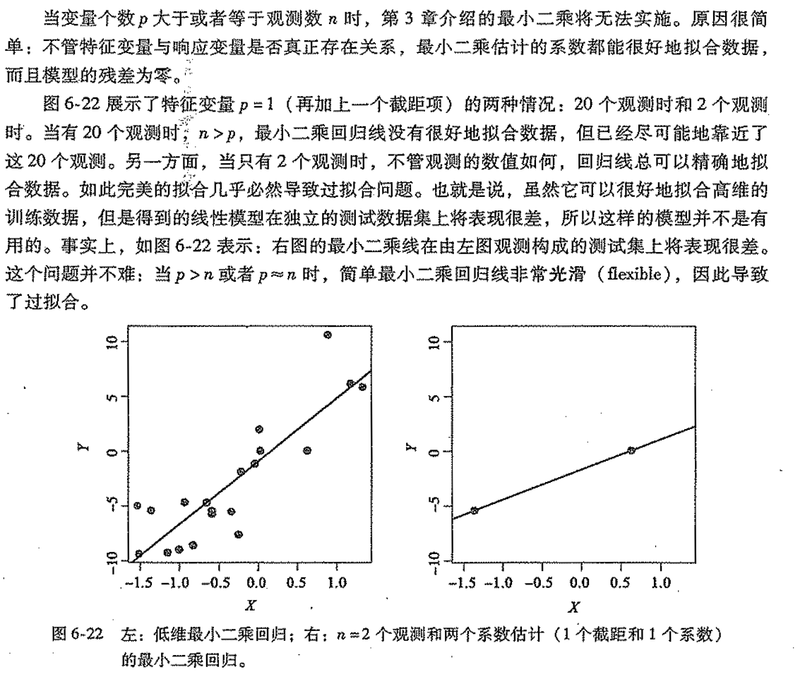
• Def: problem2

  

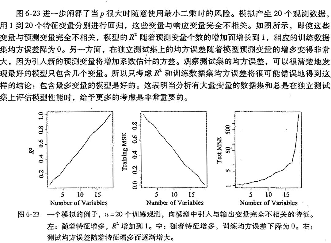
• Def: problem3

  

  

  

  

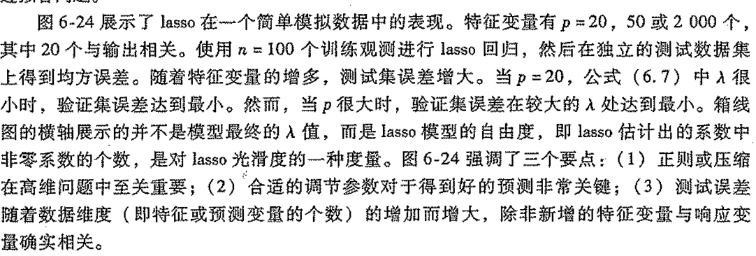
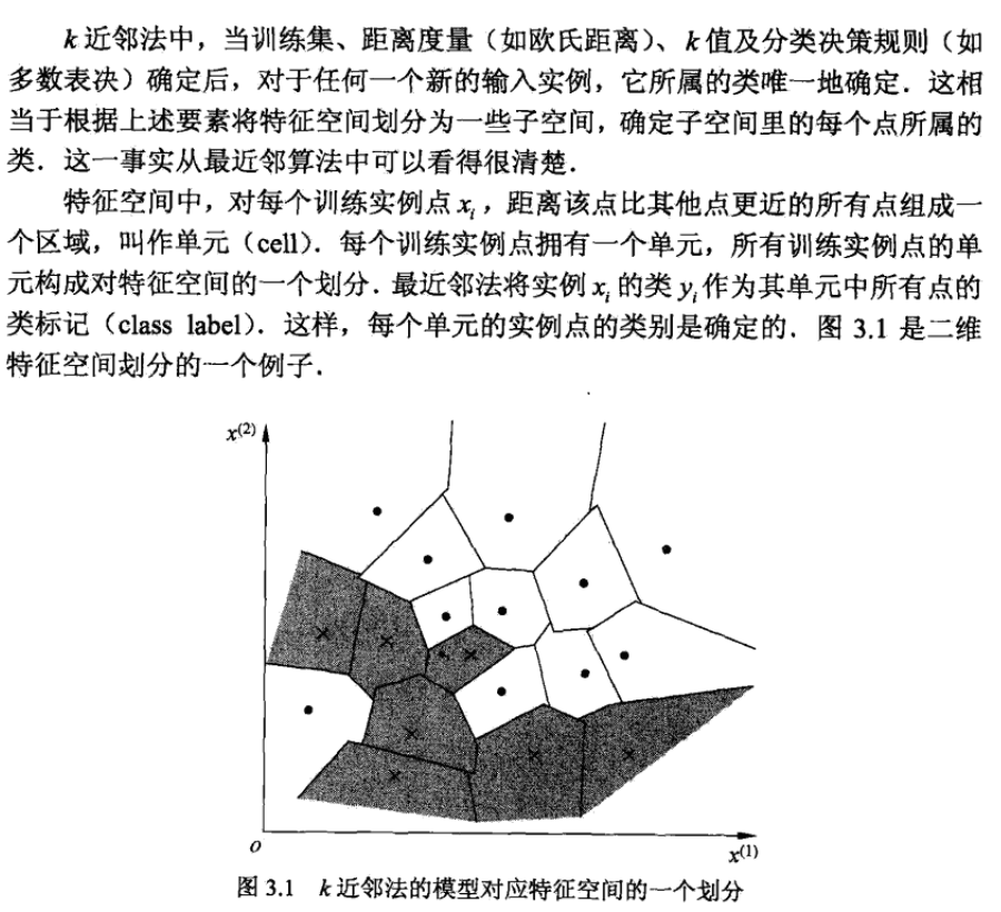
2.2. knn algorithm

• Usage: discriminative model

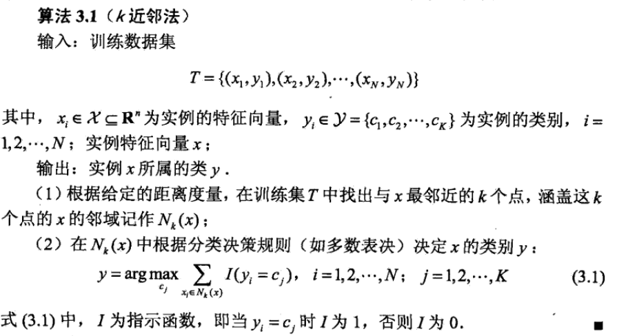
• Def: choose the most appeared class in x's neiborhood

  $$ p(y=c_j|x) = I[c_j=c {x_i N_k(x)}^{} I(y_i=c_j)]

  $$

  

  • Note:

    

2.2.1. loss function

• Def: 0/1 loss function

  \[ L(f, x, y))=I[y \neq f(x)] => E(L(Y,f(X))) \]

  

  • Note: how to reach \(f\): preset structur: neighbor voting
  • note: how to get res: intuition.
  • Note: how to reach \(\hat{f}\): to minimize EmL, we find that if we use the result from dataset \(\sum_{x \in N_{k}(x)} I\left(y_{i}=c_{j}\right)\) then it is equivalent to trainning EmL(f, X, Y).

2.2.2. alternatives & improvements

2.2.2.1. distances

• Note: different distances

  

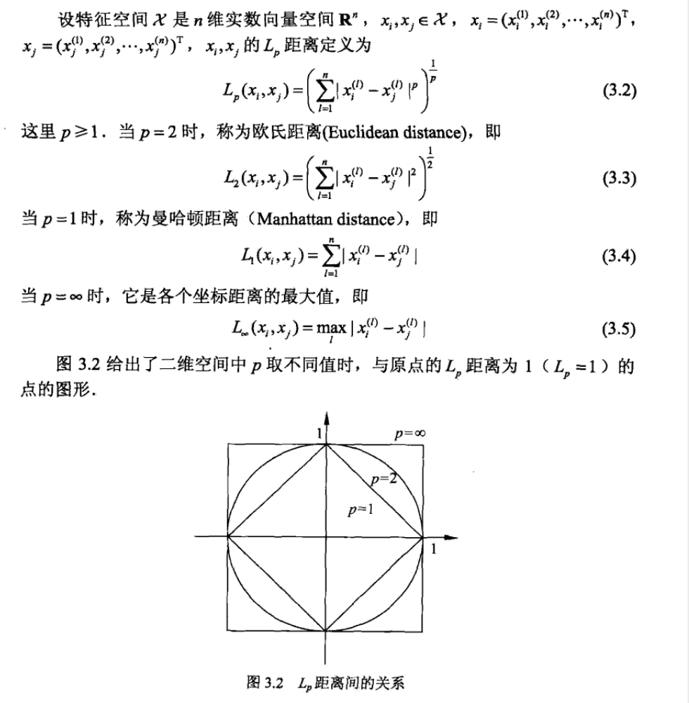
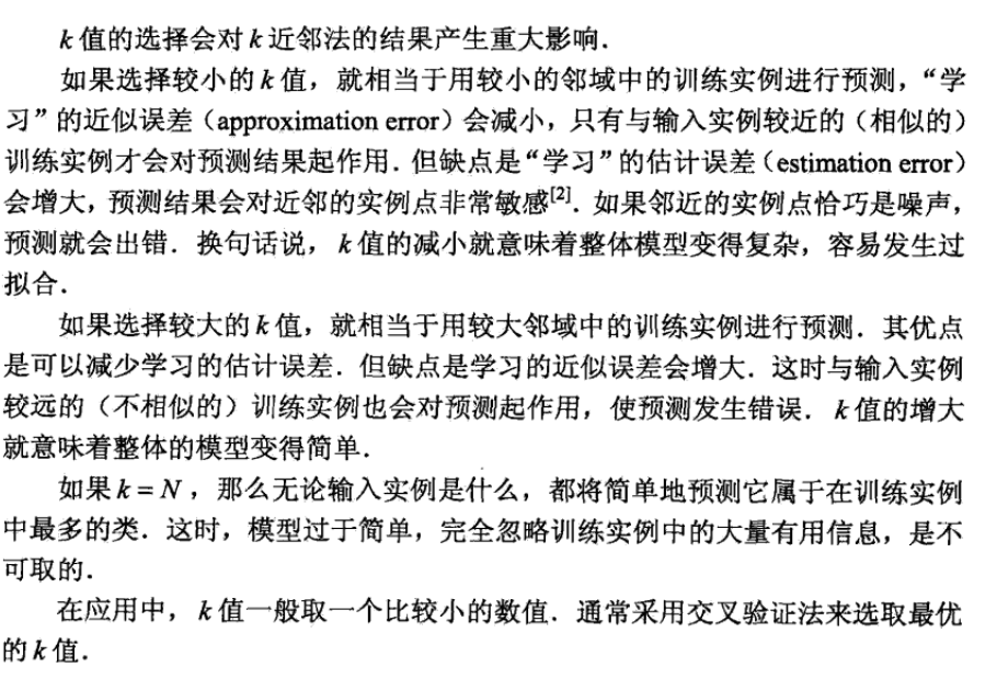
2.2.2.2. choose of k

• Def:

  

  2.2.3. implementation

• Def: kd tree

  

• Def: how to build

  

  

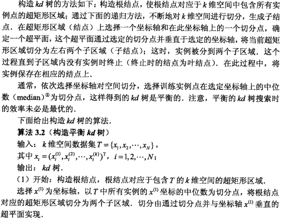
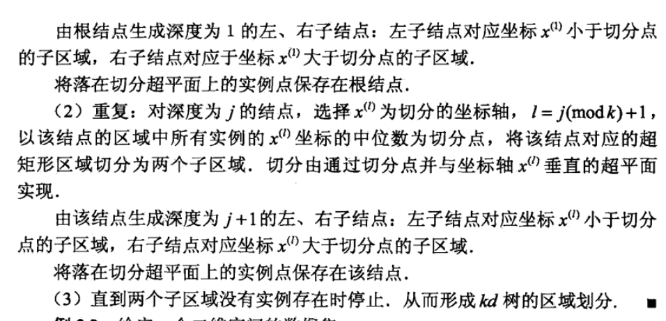
  • Note: 1 layer => 1 dimension, 2 layer => 2 dimension, ...

  • Note:

    

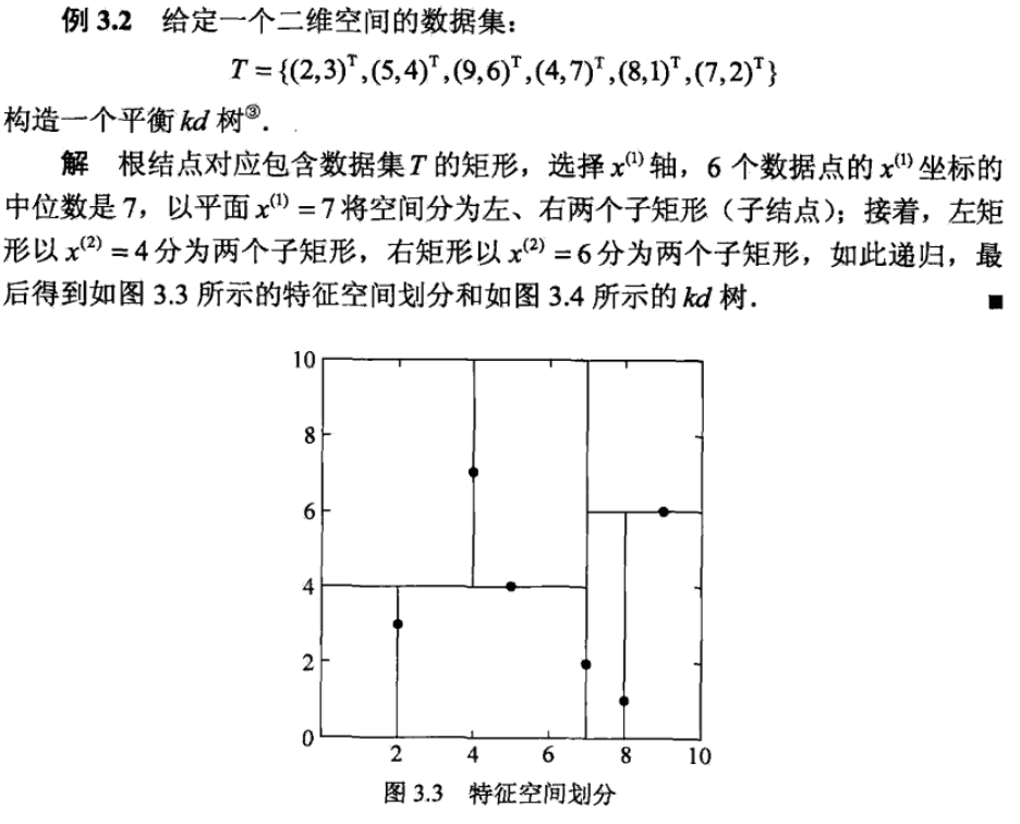
• Def: how to use kd tree

  

  

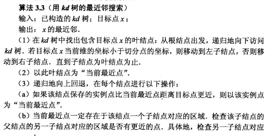
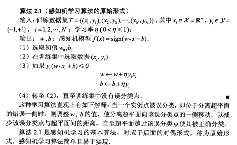
2.3. perceptron algorithm

• Usage: discriminative model

• Def: The perceptron algorithm performs pattern classification when F is the class of linear threshold functions.

  $$ p(y=1|x) = I[f(x)=sign(w ^{T} x)>0]

  $$

  

• Def: how to build

  

  • Note: figure of perceptron

    

    • Qua: One important feature of this algorithm is that it only uses inner products of the data points.

      let, where \(n_i\) is the time that \(x_i\) gets updated.

      \[ \alpha_i = n_i \eta \]

      so we have

      \[ w_N = \sum_{n=1}^{N} \alpha_i y_i x_i \\ b_N = \sum_{n=1}^{N} \alpha_i y_i \]

      the prediction rule becomes

      \[ \hat{y}_i = sign(w_N ^{T}x _{i}+b_N) = sign( \sum_{j}^{}a _{j}x _{j} ^{T} y_jx _{i}+b_N) \]

      updates becomes (i is one of the misclassified points)

      \[ a _{i} ^{(t+1)} = a _{i} ^{(t)} + \eta \]

      

      • Note: from this quality we can see the inspiration of kernel, that we only need the inner product of xixj, with the quality of readiness of computing inner product after projection, we can use kernel to get a more complex model

        

2.3.1. loss function

• Def:

  \[ L(w,x,y) = -y(wx+b) I[f(x)y<0] =>-\sum_{x_{i} \in \mathbb{M}} y_{i}\left(w \cdot x_{i}+b\right) \]

  

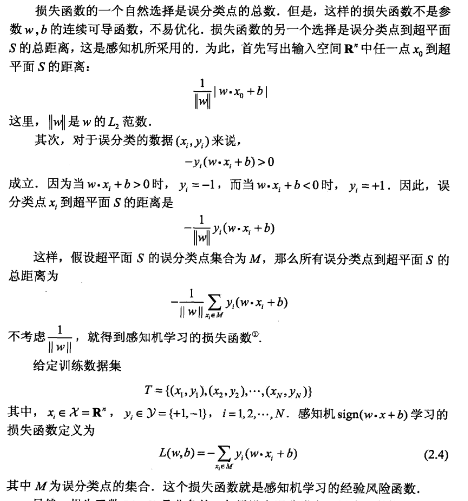
  • Note: how to reach \(f\): preset structure: linear model

  • note: how to get res: intuition.

  • Note: how to reach \(\hat{f}\): minimizing EmL: which is distances of mis classified nodes, we want them to classify correctly=>loss=0. note that we don't use the normal loss functions. Training = partial gradient descent(point by point).

2.3.2. optimization algorithm

• Def:gradient descent

  

  

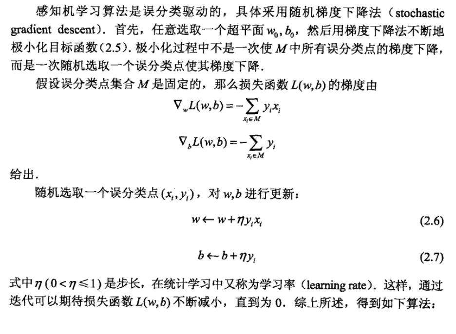
2.3.3. convergence

• Theorem: complexity of the algorithm to converge.

  • Usage: result gives a bound on the number of steps in terms of some properties of the data.

    

  • Note: perceptron complexity may not be linear, it is possible it do not terminate after a long time

    

2.3.4. evaluation

• Lemma: linearly independent => seperatable data

  

  Proof:

  

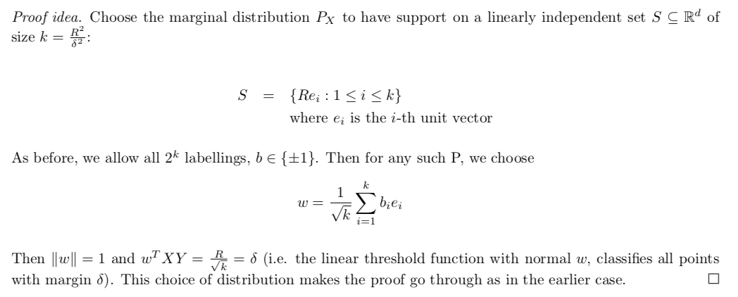
  • Theorem : The main theorem in this section shows that for any prediction rule (from the class of linear threshold functions), there is a probability distribution that is linearly separable, but for which the prediction rule does poorly when averaged over all training data sets.

    Usage: we can compute this lower bound, to estimate the risk for this threshold function.

    

    Proof: too long

    Note 1: see this bound as minimax lower bound, meaning that whatever \(f _{n}\) you choose, there exists some part of the training dataset that yield result with lower bound.

    

    Note 2: generalization using VC dimension.

    

• Theorem: If we restrict our attention to probability distributions that have a large margin, we can prove an upper bound for the risk of the perceptron algorithm:

  

  Proof:

  

• Theorm: In the above theorem, we were maximizing over all probability distributions. If we restrict the maximization to be over those probability distributions having a large margin we can obtain a better lower bound:

  

  Proof:

  

2.4. support vector machine

• Usage: special form of perceptron(same structure) where distance is maximized.

• Def: function distance1

  

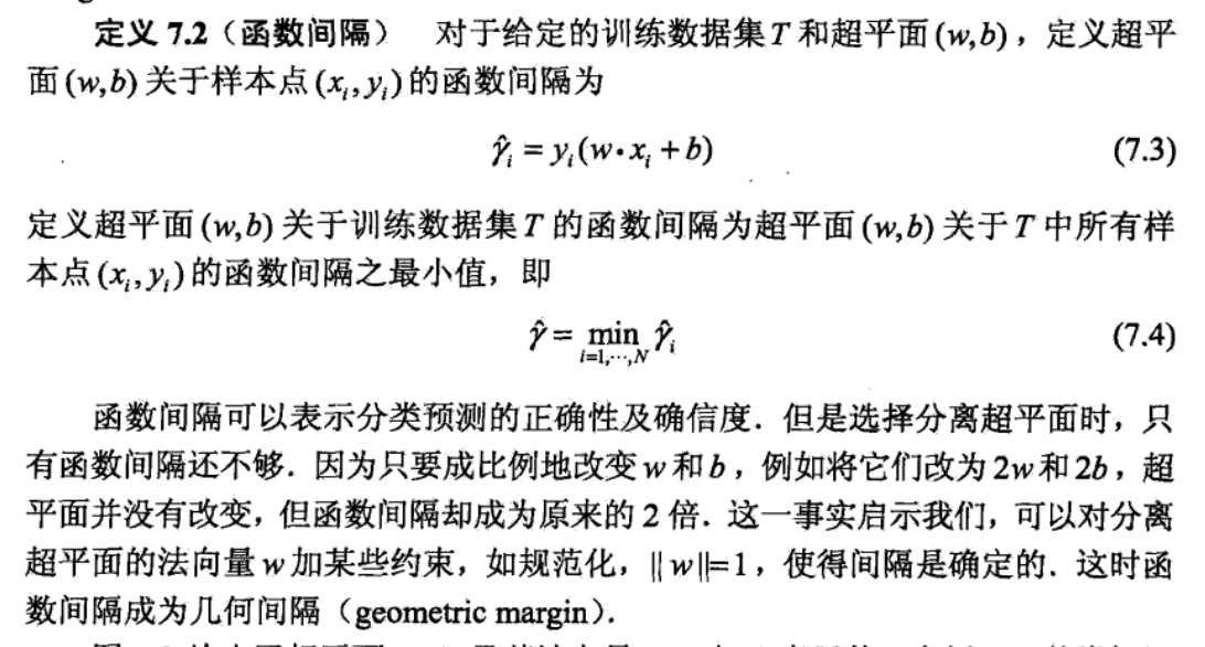
• Def: geometry distance

  

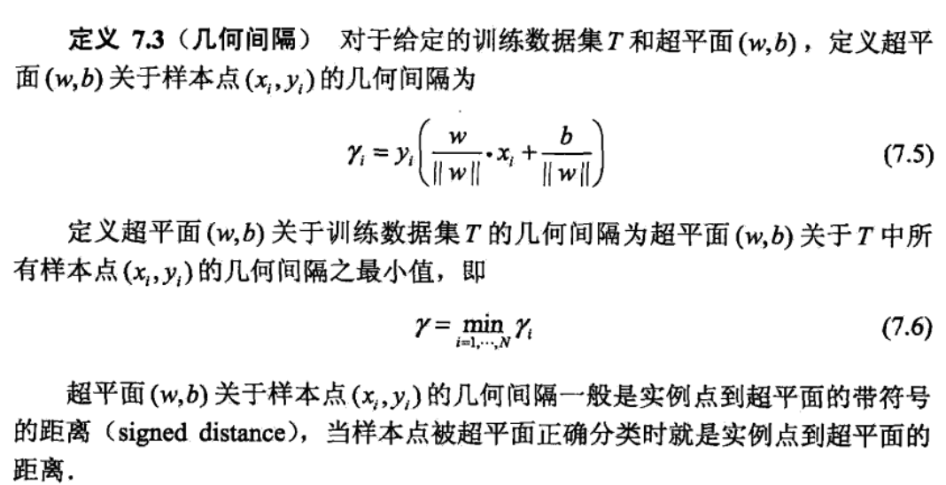
  • Qua: relation ship with distance 1, we know that geometry distance is not affected by w alone.

    

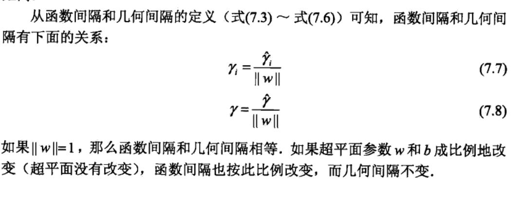
• Def: support vector machine model

  $$ p(y=1|x) = I[f(x)=sign(w ^{T} x)>0]

  $$

  

  • Note:

  

2.4.1. loss fucntion

• Def: loss function for soft C, if hardmargin(basic form), lambda = 1/infinity

  \[ L(w,x,y) = ||w||^2+[1-y(w*x+b)]_+ =>\sum_{i=1}^{N}\left[1-y_{i}\left(w \cdot x_{i}+b\right)\right]_{+}+\lambda\|w\|^{2} \]

  

  • note: that [1-x]+ vs I(x)x>0. 这里I[x]可以用于可分，因为它最少就是0，是0的时候就是可分的。同理我们也可以用硬间隔把[1-x]+前面的系数调成正无穷，那么效果是和I[x]一样的。只不过我们多加了||w||这项，这项是为了最大化间隔。
  • note: how to get f: preset, linear model
  • note: how to get res: intuition.
  • note: how to get \(\hat{f}\) : by minimizing EmL: mimizing not only the misclassified distance(hinge loss), but also the parameter to make distances as large as possible, training = optimization(IIS. newton).

2.4.2. optimization

2.4.2.1. basic

• Qua: basic transformations

  trans: other form \(\left \| w\right \|=1\)

  

  MWpfw8.png

  trans: other form \(\left \| w\right \|=1/ \gamma\)

  

  MWpOmV.png

  overall

  

2.4.2.2. dual

• Def:

  lagrange function

  

  goal: max min

  

  get lagrange dual problem ( solve the min problem)

  

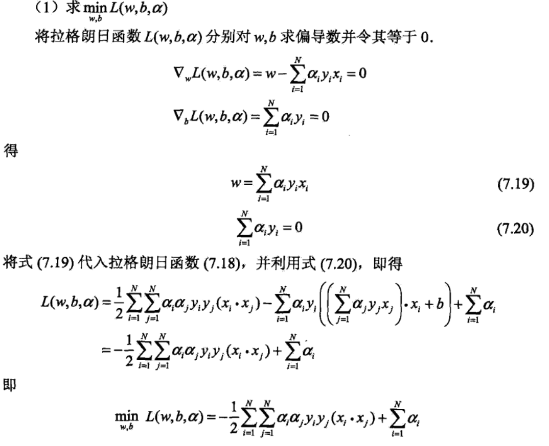
  final: solve lagrange dual (max problem)

  

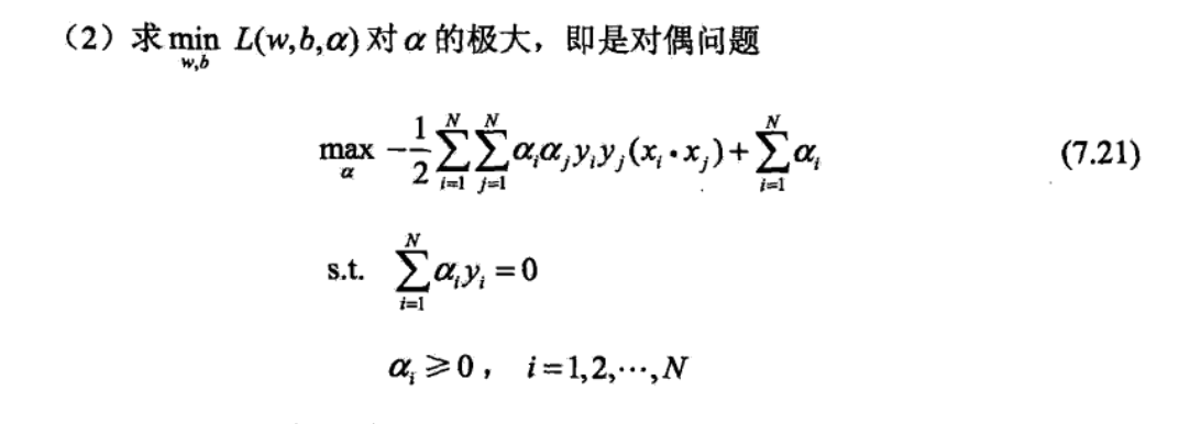
  recall slackenss for dual problem, this show that the those with ai(penalty loss) \(\neq\) 0, are exactly those in the margins. 算法解只由支持向量决定。

  

  recall the kernel stuff, we can use kernel to efficientlly solve this, for more kernel stuff turn to 2.2.2

  

  overall

  

  

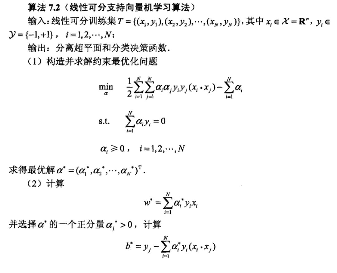
2.4.3. alternatives & optimization

2.4.3.1. kernel SVM

• Def: dual problem & kernel function

  dual problem (only inner products determines solution)

• Qua: kernel function can reduce complexity of dual problem.( further discussion can be find in linera algebra)

  Usage: 由此看出，即使没有kernel，只要找到映射关系，我们仍然可以实现低维空间映射到高维空间，进而通过高维向量内积运算来寻找最佳分割超平面。但是，kernel的引入，降低了向量内积运算的计算复杂度。无论我们映射到几维空间，我们只要把原有维度代入核函数，就能等价于高维上的内积运算。极端的情况下，特征空间映射到了无穷维度空间，如果没有核函数，根本无法计算出映射后的向量内积。

  （映射到新的特征空间后的内积=原空间核函数）

  https://blog.csdn.net/zhangjun2915/article/details/79261368

  k(xi, xj) is the kernel function of inner product of xi, xj

• Def: kernel function

  

  

  • Note: k = HxH->R, we project nodes to higher dimension and do SVM in higher dimension, the results are got by kernel inner project.

  • Example:

    

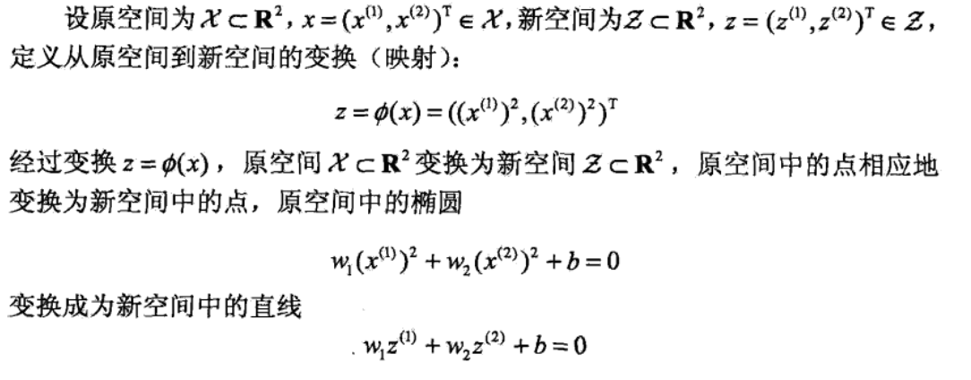
  • Example: polynomial kernel

    

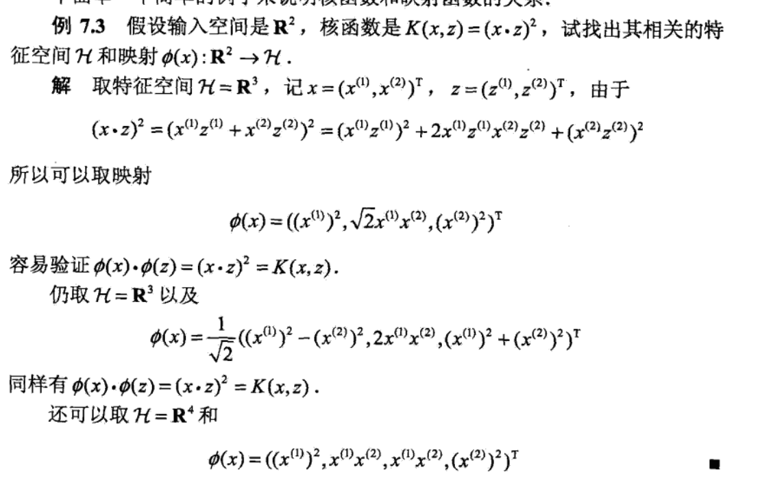
  • Example: gaussian kernel

    

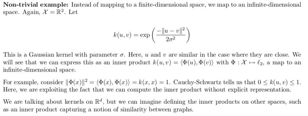
  • Theorem: what kind of K is kernel(can be split

    

• Def: f is a function space : R->R

  

  • Def: inner product on S: SxS->R

    

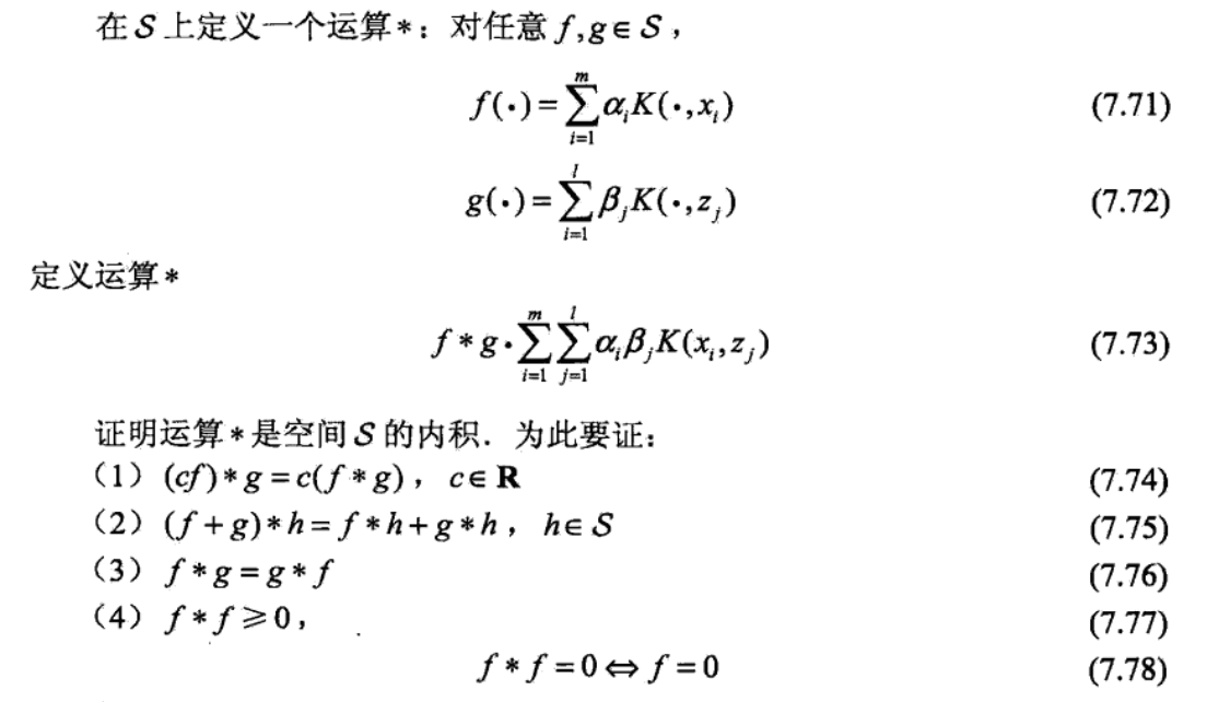
  • Qua: the definition of f and innerproduct makes S a RKHS. S is a space (\(\phi\), K, f, ), where f & are self-defined function & inner product. note that this quality does not come from K or \(\phi\), K could be any thing, RKHS comes from (f, *).

    

• def:

  

2.4.3.2. primitive SVM

• Usage: a more natural way

• Def: primal SVM,

  

  lagrangian functiion

  

  getting lagranian dual function

  

  lagrangain dual function

  

  dual problem

  

  this problem can actually be solved by hand: first solve \(\beta = \sqrt{1/4 \left \| \sum_{i}^{}\lambda _{i}y _{i } x _{i}\right \|}\), then we get the following

  

  interpreting results

  

2.4.3.3. soft C-SVM

• Usage:

  

• Def: soft SVM

  

• Qua: basic transform

  trans: change |x<1| to (1-x)+ , basiclly is the same .

  

  trans: slack variable

  

  

  lagranrian function => dual lagranian function (solve min)

  

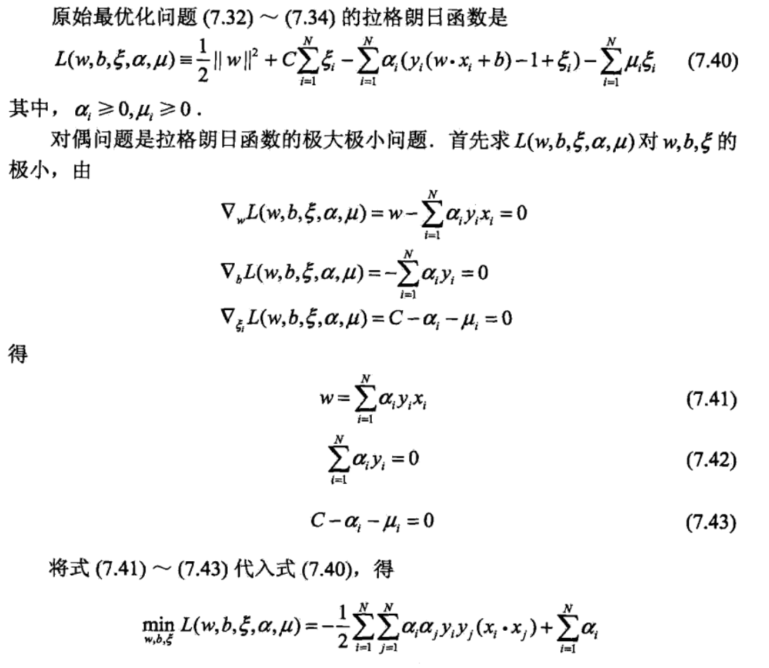
  dual problem (solve max)

  

  

  

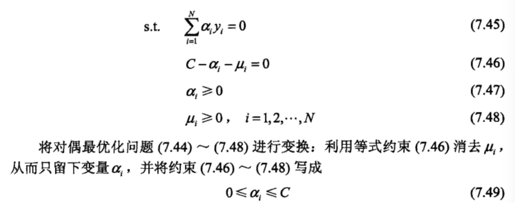
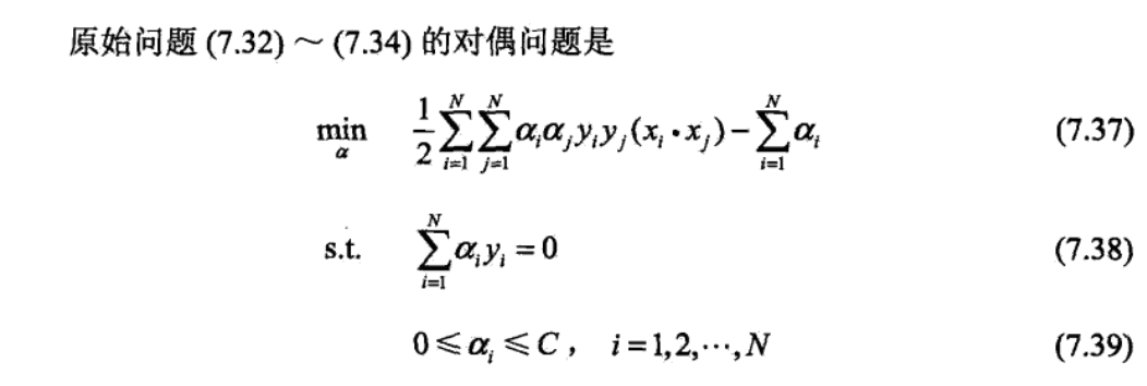
  choose c

  

  overall

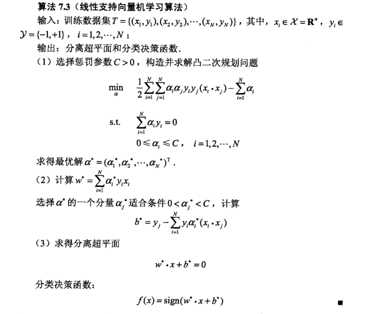
  • Note: photo of soft support

    

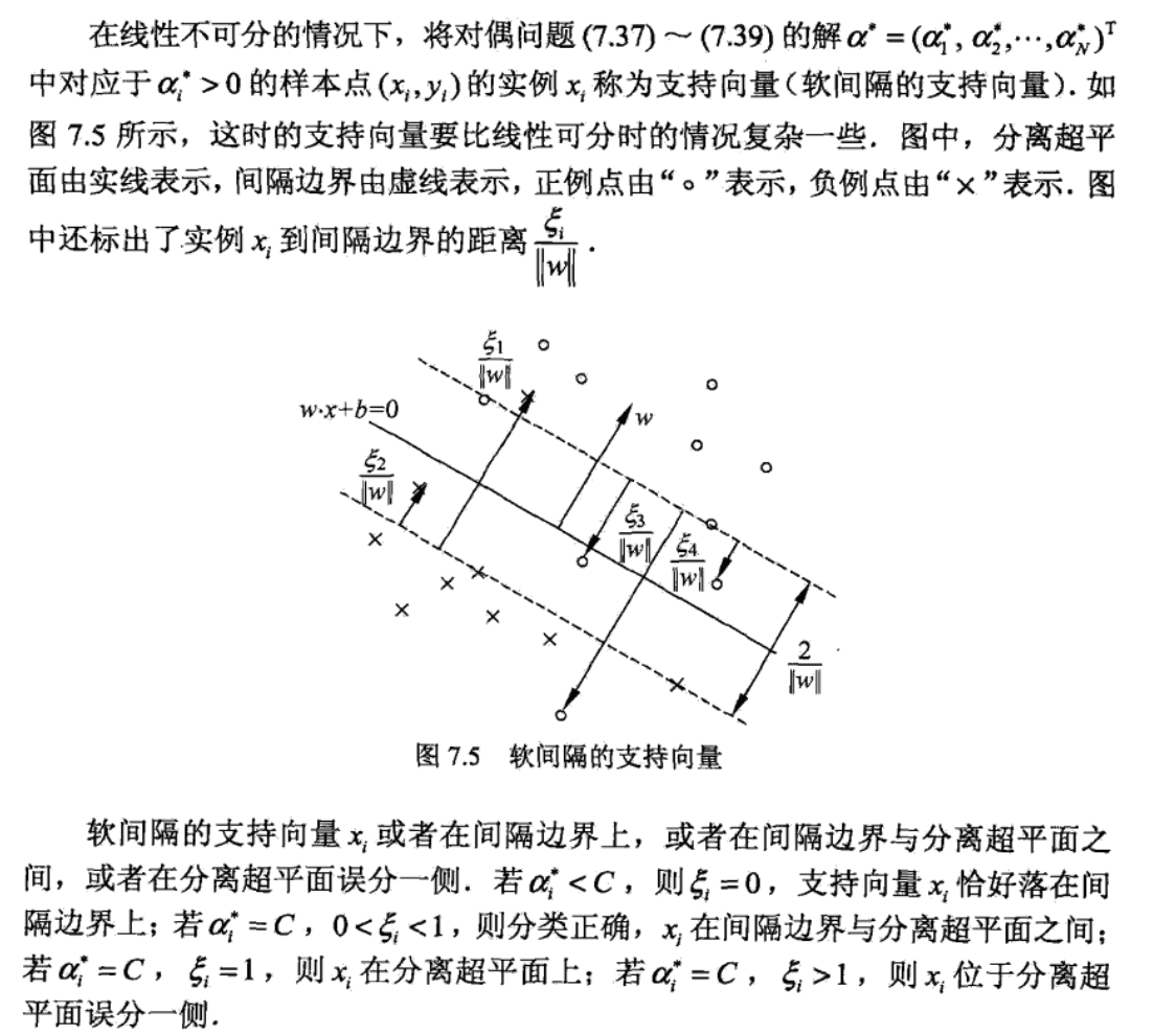
• Qua: interpreting in another way( loss function + regularization)

  

2.4.3.4. soft $ $-SVM

• Def: a more interpretable way, since \(\nu\) is more easy to set.

  

  • Qua: basic transition

    slack variables

    

    lagrange dual function

    

    dual problem

    

    insights for slackness

    

  • Qua: interpretation of \(\nu\) : we can interpret \(nu\) as being approximately the fraction of data that are margin errors.

    [](/Users/huangbenson/Library/Application Support/typora-stats_theory(https://tva1.sinaimg.cn/large/006y8mN6ly1g94litz5uxj316604g3zx.jpg)

• Qua: \(\nu\) and C SVM are the same

  

  Proof:

  

2.4.3.5. $ $-sensitive SVM (1-10)

• Def: a relaxation of loss function

  

2.4.4. convergence

• Theorem:

  

2.4.5. relationship with logistic regression

• Def:

  

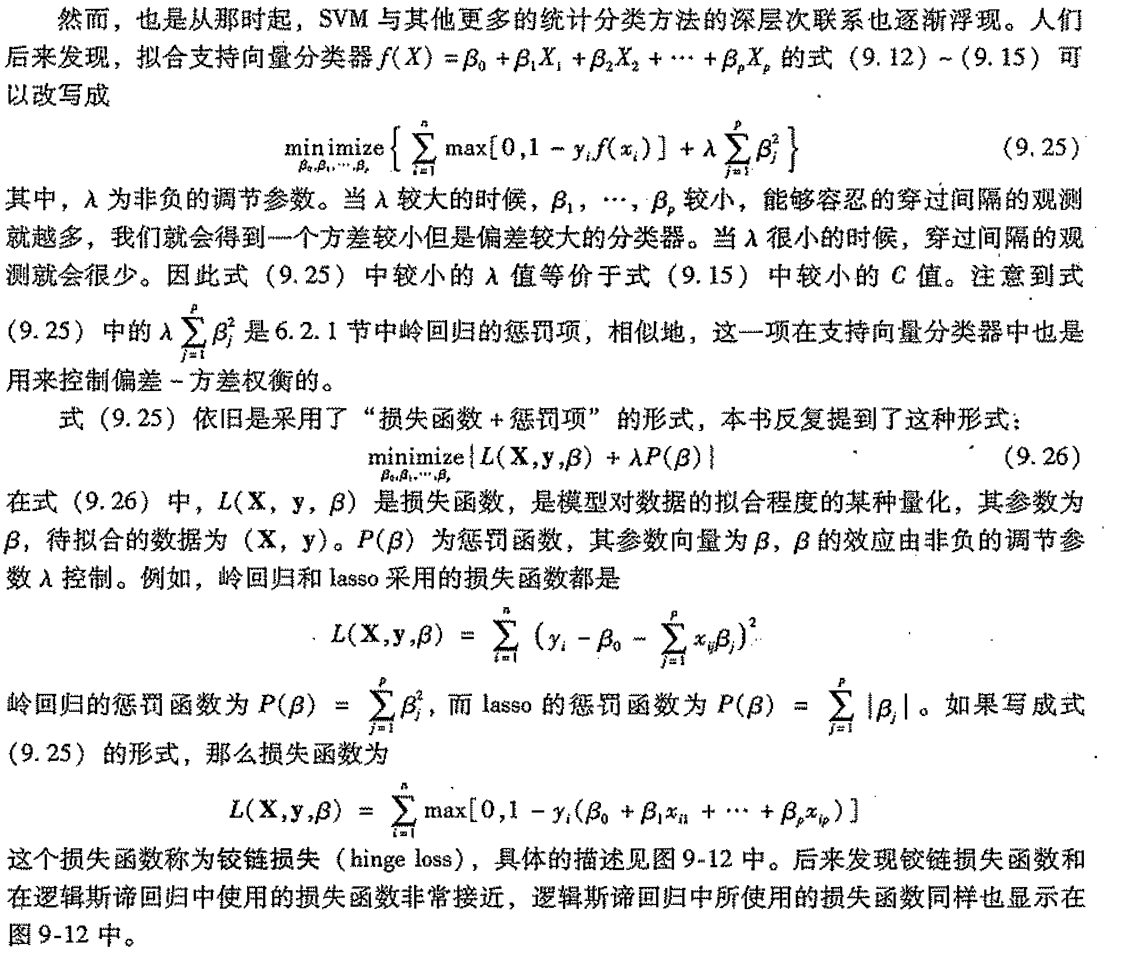
  • Note:

    

    

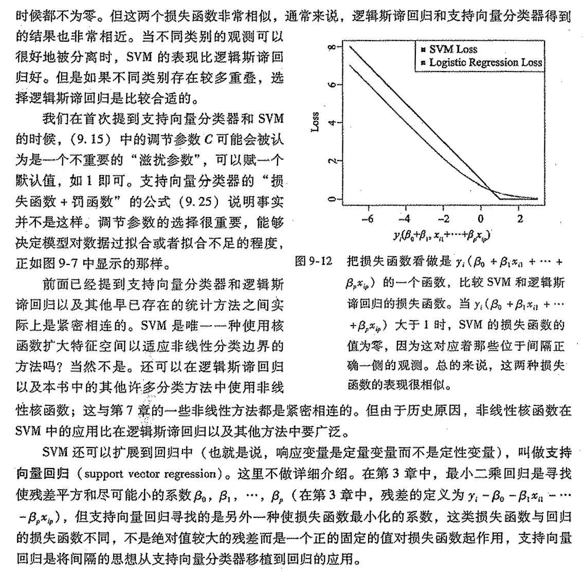
2.5. discriminant algorithm

2.5.1. LDA: by distance

• Def: distance

  \[ p(y=m|x) = I[d(x,G_m)=min_m] \]

  

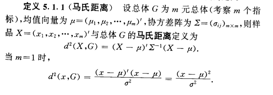
• Algorithm:

  

  • note: f preset structrue, minimize distance

  • note: f ha comes from computing parameter of dataset=>distance

2.5.1.1. if \(\sum1 = \sum 2\)

• Algorithm:

  

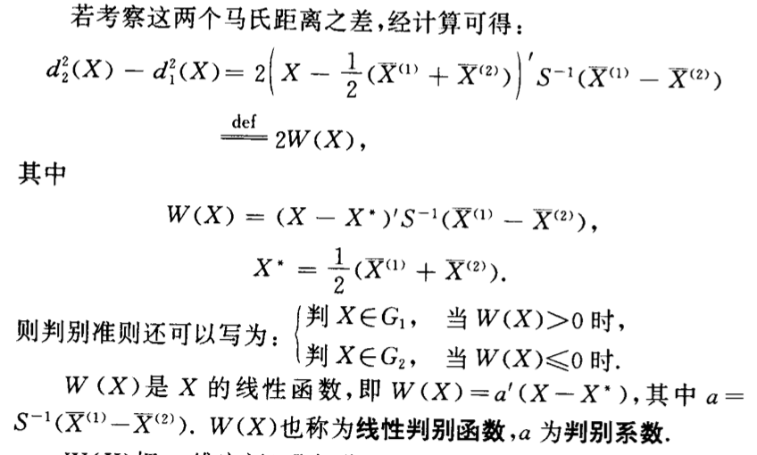
2.5.1.2. if \(\sum1 \neq \sum2\)

• Algorithm:

  

  

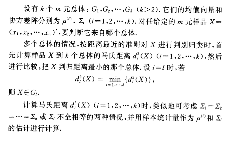
2.5.1.3. if more than 1

• Algorithm:

  

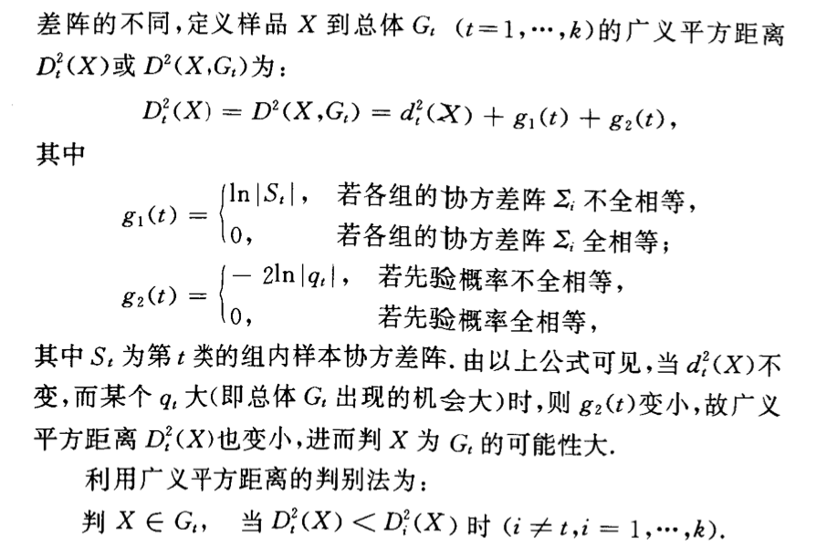
2.5.2. QDA: by general distance

• Algorithm:

  

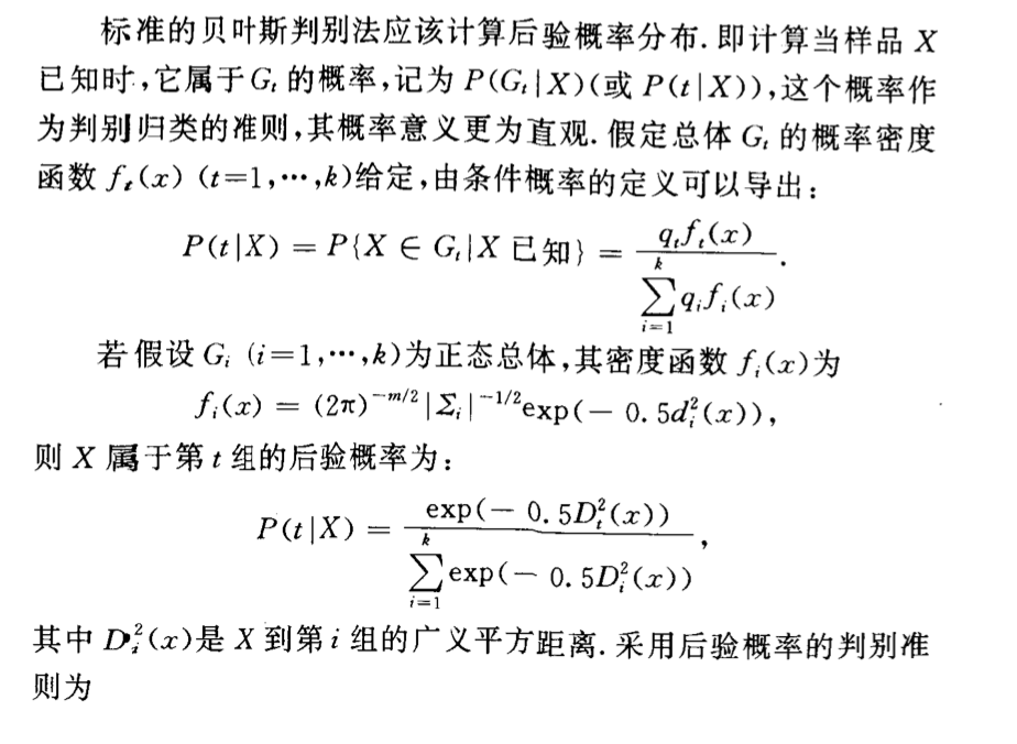
2.5.3. by max posterior (estimate)

• Algorithm: not similar to logistic, logstic is a distribution in whole & linear model, not using full probability expansion. This is similar to bayes => except this is exp normal model, bayes is discrete.

  

  

2.5.4. by bayes

• Def:

  

  

• Def: miss classification loss

  

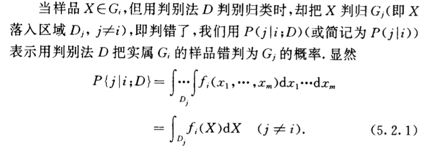
• Def: total miss classification loss

  

• Theorem: the main theorem of bayes classification

  

  

  Corollary:

  

2.5.4.1. if \(\sum\) all the same (gaussian)

• Algorithm:

  

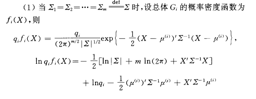
2.5.4.2. if not all the same (gaussian)

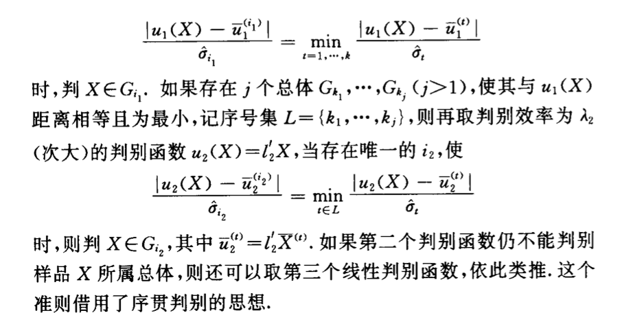
2.5.5. by Fisher

• Def:

  Usage: adding projection procedure to separate the data.

  

  

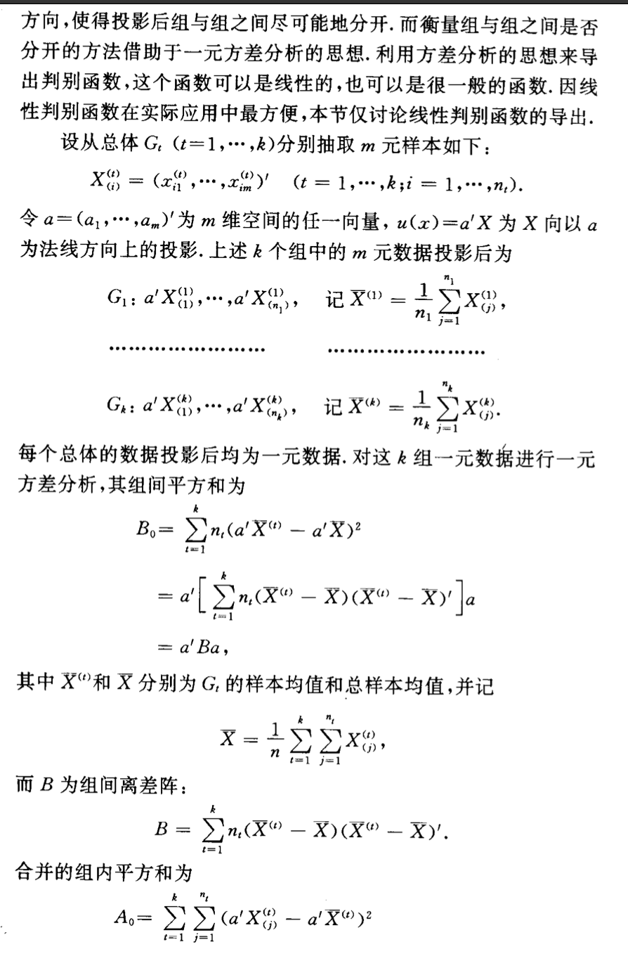
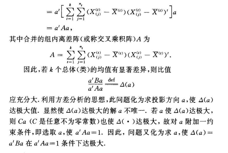
• Theorem: the best direction

  

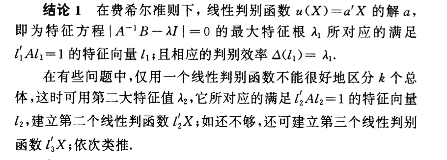
2.5.5.1. r=1

2.5.5.1.1. k=2

• Algorithm:

  

2.5.5.2. r=?

• Algorithm:

  

  

2.6. bayes algorithm

• Usage: generative model

• Def:

  \[ P\left(Y=c_{k} | X=x\right)=\frac{P\left(Y=c_{k}\right) \prod_{j} P\left(X^{(j)}=x^{(j)} | Y=c_{k}\right)}{\sum_{k} P\left(Y=c_{k}\right) \prod_{j} P\left(X^{(j)}=x^{(j)} | Y=c_{k}\right)}, \quad k=1,2, \cdots, K \]

  

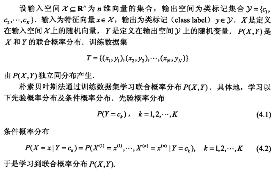
  • Note: we have to assume that X is independent in every dimension（every dimension is a feature)

    

• Def: using kernel to interpretate

  

2.6.1. loss function

• Def: 0/1 loss

  \[ L(f,x,y)=I[{y \neq f(x)}]=>E(L(Y,f(X))) \]

  

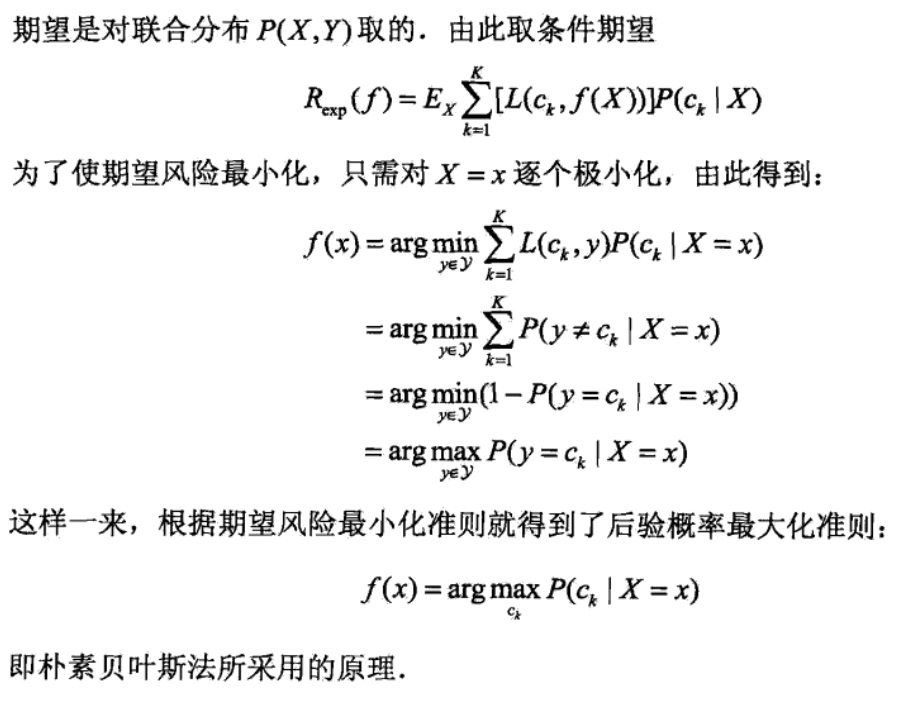
  • Note: how to get f: bayes does not have a presumed structrue like perceptron / knn, it(f) derives from the basic rule of conditional probability
  • note: how to get res: it derives from minimizing EL with 0/1 loss function. Actually every algorithm that uses argmax post probability is minimizing EL.
  • Note: how to get \(\hat{f}\): instead of minimizing EmL, we use max likelihood to get $ $.

2.6.2. optimization algorithm

• Def: max likelihood

  

  

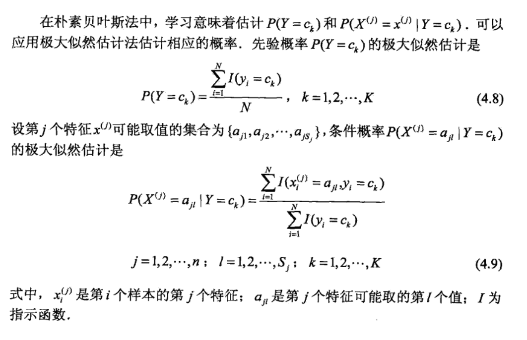
  • Note: that here we assume discrete feature of X, and the derivation is here : https://blog.csdn.net/weixin_41575207/article/details/81709379

  • Note: example

    

    

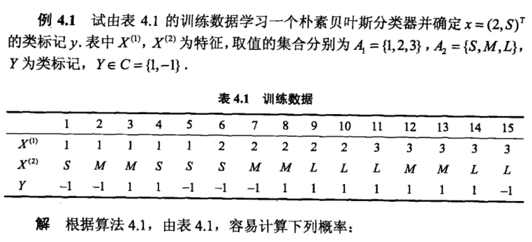
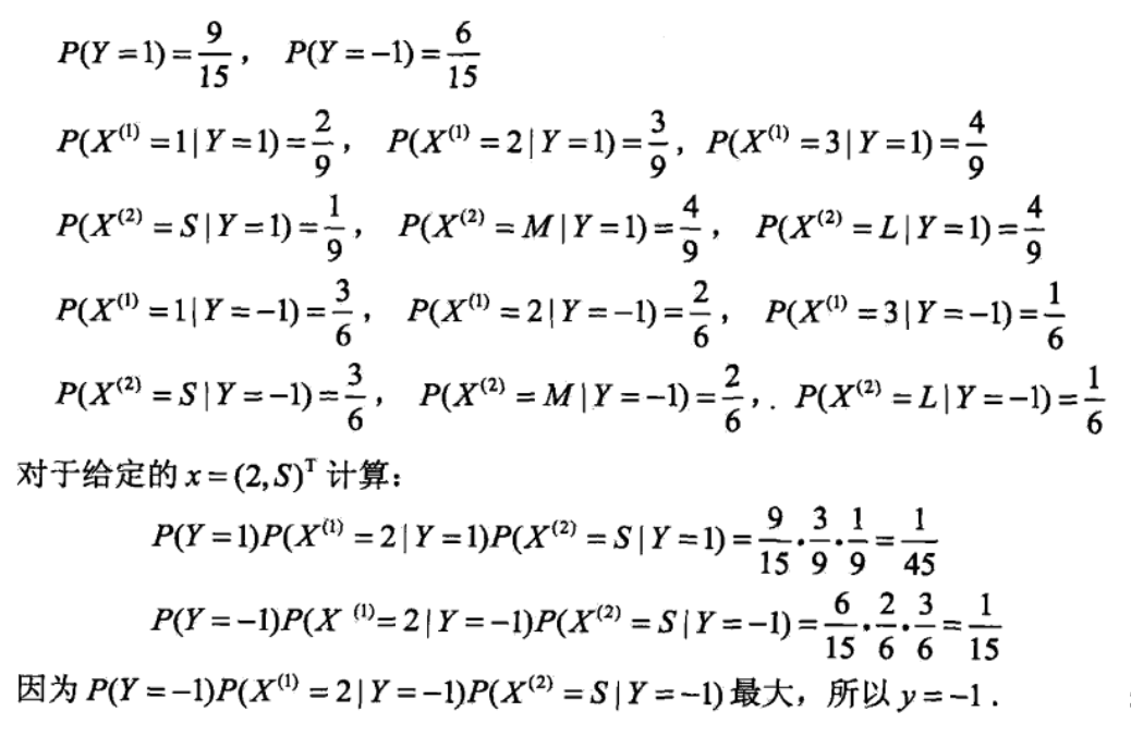
2.6.3. alternatives & improvements

2.6.3.1. laplace smooth

• Def: laplace smooth

  

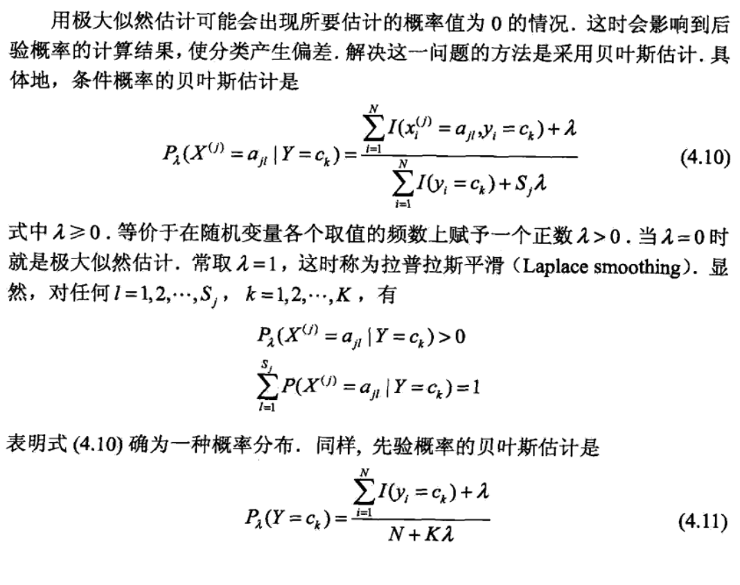
  • Note: example

    

2.7. logistic regression (1-13)

• Def: distribution

  

  • Note:

    

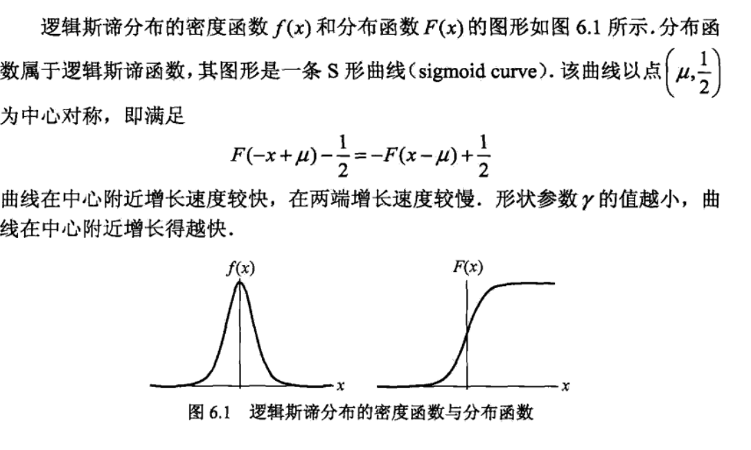
• Def: logistic regression model

  \[ P(Y=1 | x)=\frac{\exp (w \cdot x+b)}{1+\exp (w \cdot x+b)} \]

  

  

• Def: logit = log(p/1-p)

  

2.7.1. loss function

• Def: loss function = - log(likelihood)

  \[ L(f,x,y) = -log( \prod_{i=1}^{N}\left[\pi\left(x_{i}\right)\right]^{y_{i}}\left[1-\pi\left(x_{i}\right)\right]^{1-y_{i}} ) \]

  

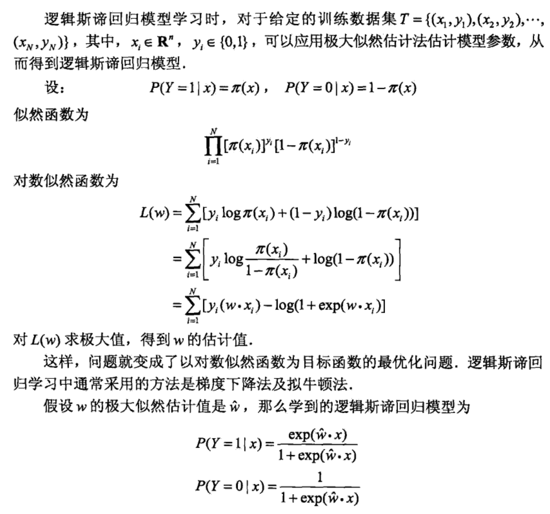
  • Note: likelihood function is p(y|x) not p(x,y) since we maximize w, adding p(x) makes no difference. In one word, we save all parts containing w.

  • Note: how to get f: preset structure: logistic distribution

  • note: how to get res: same as bayes?

  • Note: how to get \(\hat{f}\): maximize likelihood/ minimize EmL to get $ $

2.8. max entropy algorithm

• Def: special function

  

  • Qua: E

    

    

  • Qua: E is used to test if p(y|x) is empirical p(y|x)(if p(y|x) suits the dataset)

    

• Def: model

  \[ p(y|x) = f(x,y) \text{ 代求} \]

  • Note: that this model does not have any form of structure.

2.8.1. loss function

• Def: loss function

  \[ L(P,x,y) = -\sum_{x, y} \tilde{P}(x) P(y | x) \log P(y | x) \]

  

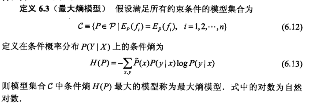
  • Note: note that this model maximize H(P) = make y as smooth & normal & equal as possible

  • Note: how to get f: no preset form!!

  • note: how to get res: same as bayes.

  • Note: how to get $ $ : use empirical conditional entropy and solve optimization problem(training), traning = optimization.

2.8.2. optimization

2.8.2.1. dual problem

• Def: this is the result of max entropy problem（p,w relationship, w still needs to be solved). Notice that this looks exactly like logistic regression.

  \[ \begin{array}{c}{P_{w}(y | x)=\frac{1}{Z_{w}(x)} \exp \left(\sum_{i=1}^{n} w_{i} f_{i}(x, y)\right)} \\ {Z_{w}(x)=\sum_{y} \exp \left(\sum_{i=1}^{n} w_{i} f_{i}(x, y)\right)}\end{array} \]

  • the original maximization problem

    

  • the minimization problem

    

  • dual problem, here we go from solving P => solving w => 把w带回P，得到P(w)，其实就是本来直接可以解P但是不好解，现在换个对偶问题解w，然后带回p和w的关系式得到P。这里的x,y指的是可能取值而不是变量。而且求导是对某一个x，y求导，这里写的是对所有x，y对求导。

    

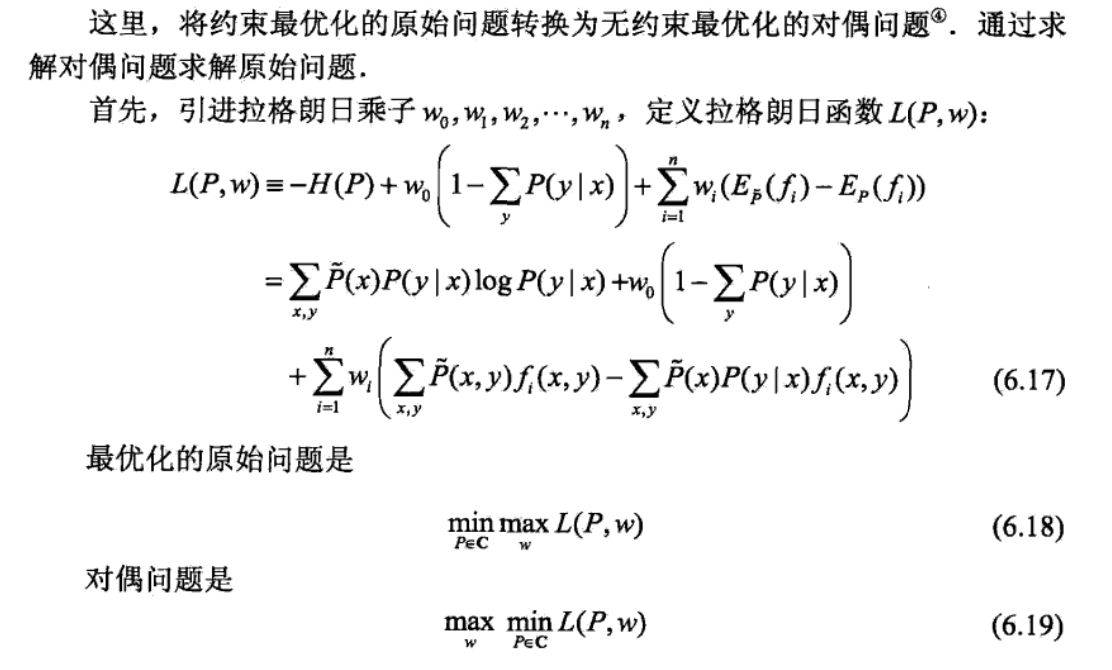
• solve min problem by first order rule, get p,w relationship. note that we get derivation with each pair of x & y, it is equivalent to getting with 1 pair.

  

  

  

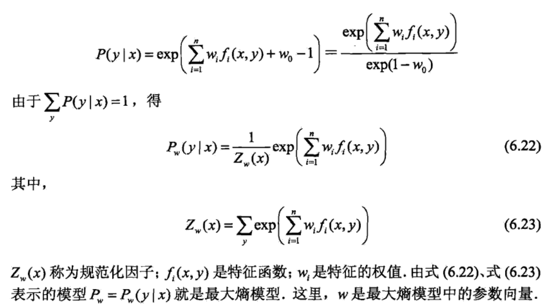
• solve the outside max problem, get w.

  

• get back p(w)

  

2.8.2.2. max likelihood

• Usage: max likelihood = max entropy

  

• Def:

  • start from likelihood function，why in this form: https://blog.csdn.net/wkebj/article/details/77965714

    

  • likelihood + p,w relationship => a function we need to maximize f(x,y,w)

    

  • dual problem => a function we need to maximize f(x,y,w)

    

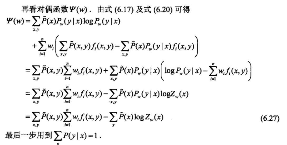
2.8.3. IIS

• Usage: similar to gradient descent

  

• Def:

2.9. ensemble algorithm

• Def: ensemble methods

  

2.9.1. boost

• Def:

  

  

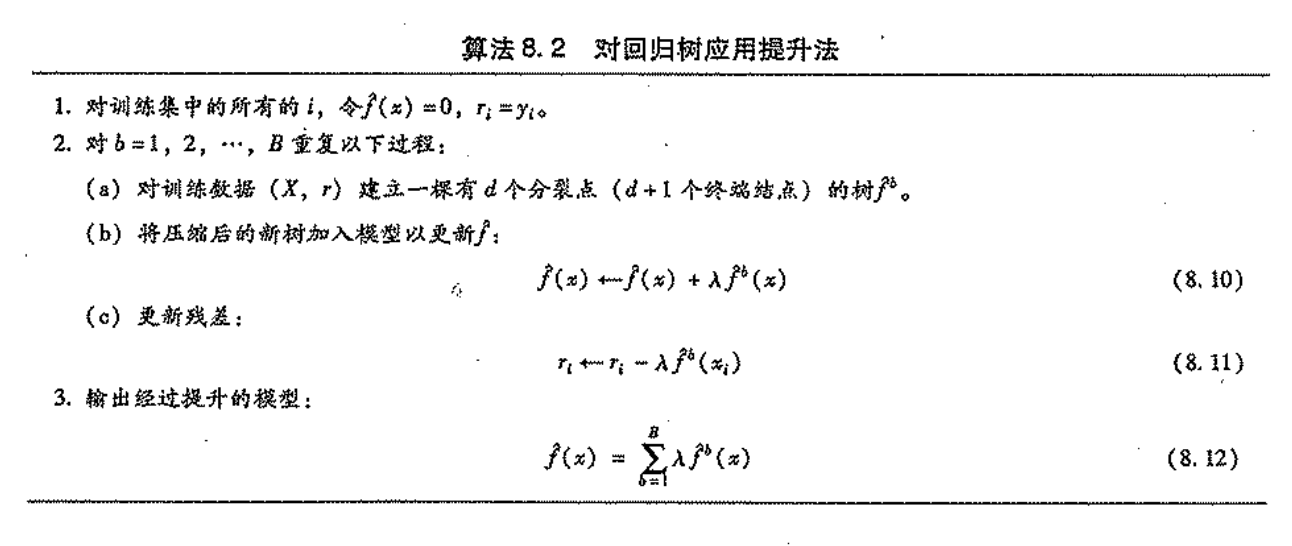
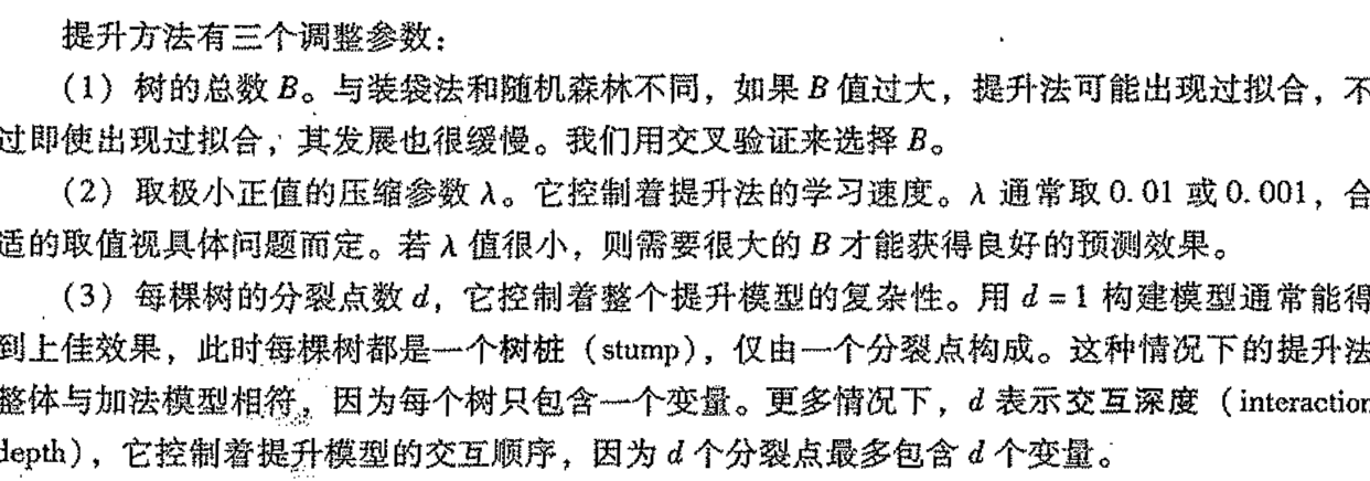
2.9.2. adaboost algorithm

• Usage:

  

• Def: adaboost algorithm

  

  

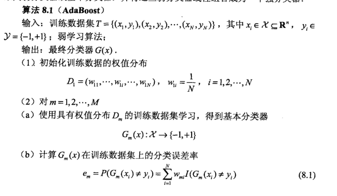
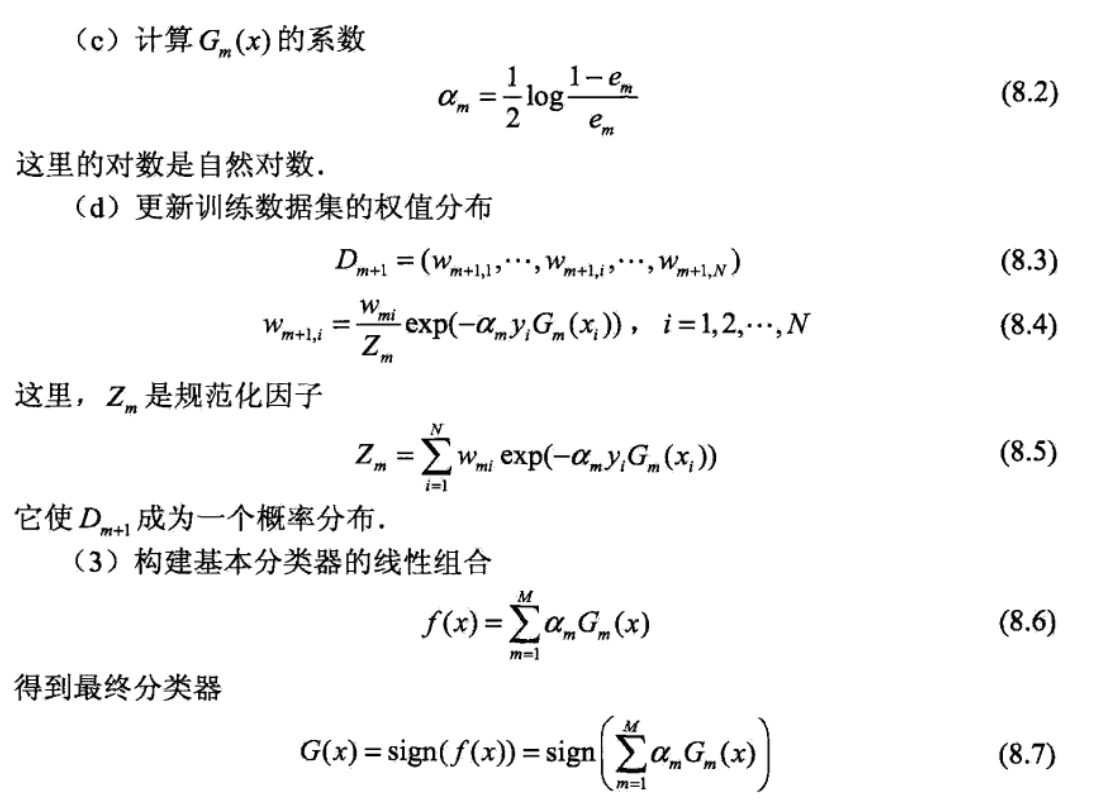
  • Note: explain why we do this way => update weight + training.

    

    

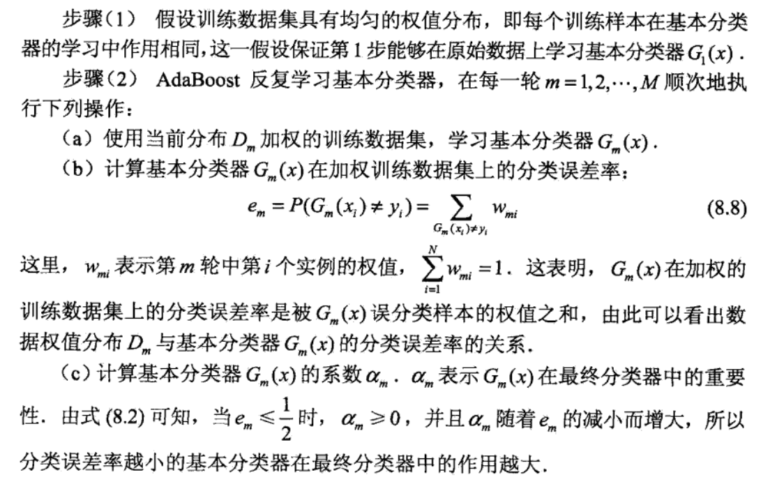
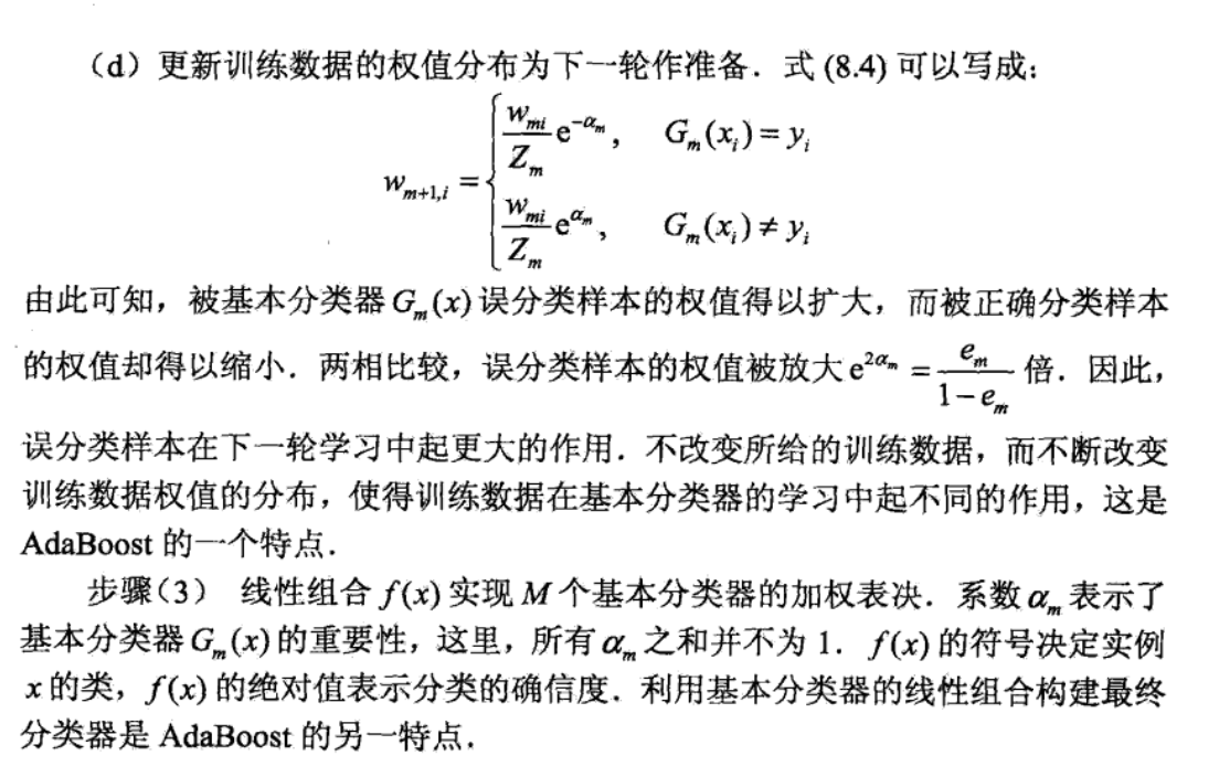
2.9.2.1. loss function

• Def: general additive algorithm

  

  

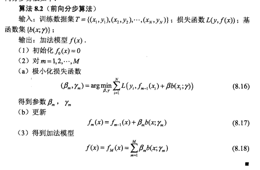
• Def: loss function = exp

  \[ L(f,x,y) = exp(-yf(x)) =>\sum_{i=1}^{N} \bar{w}_{m i} \exp \left[-y_{i} \alpha G\left(x_{i}\right)\right] \]

  

  • Note: how do we get f: from equal distribution (no preset structure)

  • note: how to get res: intuition.

  • Note: how do we get \(\hat{f}\): by optimizing exp loss function each step.（这个损失是整体的，也就是大目标就是为了让指数损失最小）

    

• Theorem: use gradient decent to explain adaboost, THIS IS THE SAME IDEA AS ABOVE

  Usage: iteratively solving adaboost is equivalent to minimizing the true loss function of \(e ^{-YF _{T}(x)}\)

  

  img

  Proof:

  

  img

  Note: loss function: For every t from 1 to T, we can expand the E(exp(-YX)) thing, and we can see that adaboost is minimizing Eexp(YFT(X)) at every step, thus the we are using step-wise gradient decent to optimize the Eexp(-YX).

  The whole picture: So this is the idea of adaboost, we choose fT to minimize eT as a step-wise gradient descent, then we find out we can see adaboost as E(-YX) in whole, so we choose \(\alpha_T\) to make that happen.

  

  img

  

  img

2.9.2.2. optimization

• Def: gradient descent .

2.9.2.3. convergence

• Theorem: there exist upper bound for loss function of each step, if database conditions are met.

  

  img

  Proof:

  

  img

• Theorem: for all classification upper bound for loss

  

  • Usage: the theory merely use update information=>tells us if we update weights in this way, how do we train Gm

    

  • Proof:

    

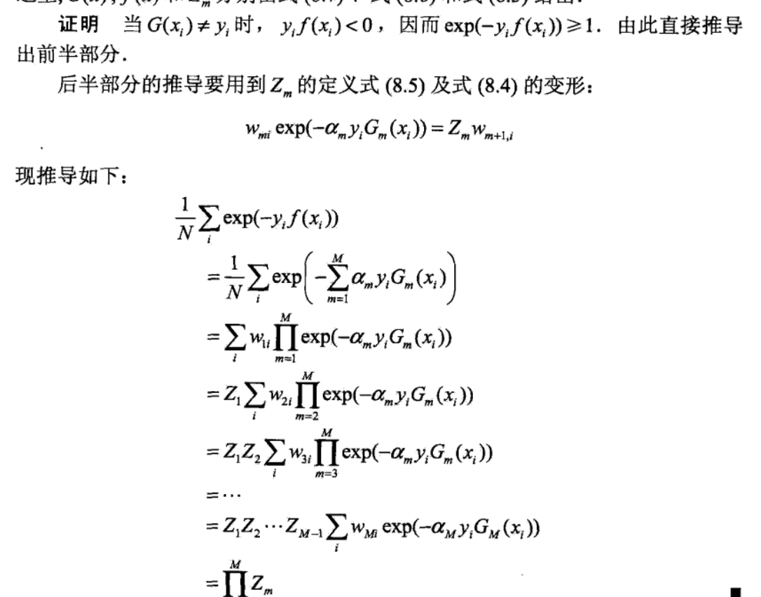
• Theorem: for 2-class

  

  • Proof:

    

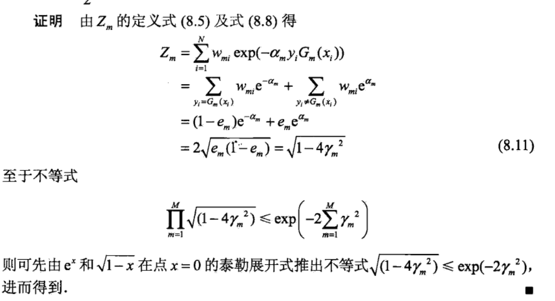
• Corollary:

  

  • Usage: if we update this way + training each round constrain \(e_m\) to a constant, then algorithm converges in exp rate.

    

2.9.2.4. alternatives & improvement

2.9.2.4.1. generalized

• Def: generalized adaboost:

  Usage: in adaboost, we use exp(-YX) as loss, here we can have different options and still implement the step-wise adaboost core idea: we see J(F) as the loss, F is the variable, and each step we take \(F+\alpha _{t}f _{t}\)

  

  img

  recall: (convex optimization)

  

  img

  Algorithm:

  

  img

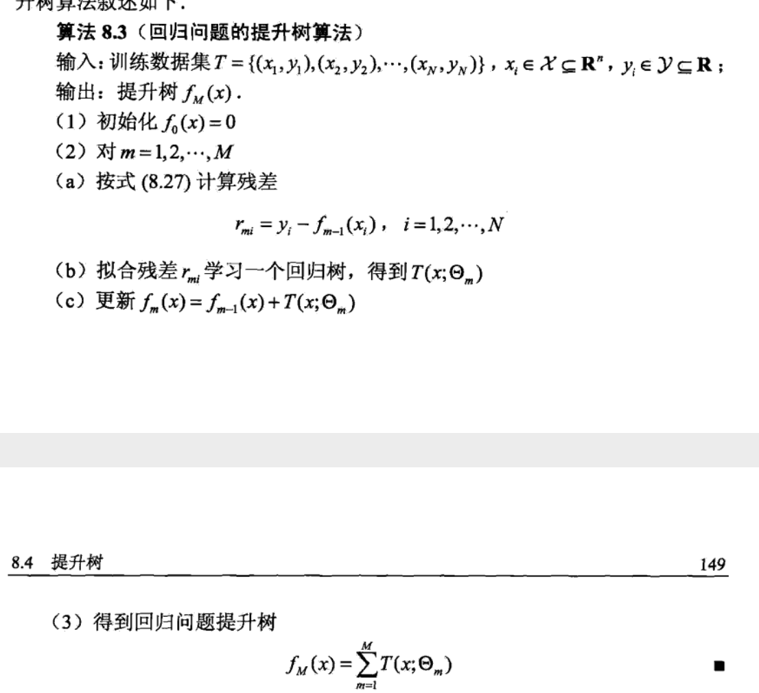
2.9.2.4.2. boosting tree

• Def:

  

2.9.2.4.3. gradient boosting

• Def:

  

  • Note: we can imagine gradient descent is using one model and doing descent by updating weight, and gradient boosting is using gradient descent by adding new model. \(f(x) = w1x+w2x+w3x\) vs \(f(x) = f1(x) +f2(x) +f3(x)\) , key point here is that f1(x) additive model is more flexible and differs from node to node even they share the same growing rate at same point(their derivative is the same).

2.9.2.5. relationship with logistic regression

• Qua: similarity to logistic regression (1-13)

  using taylor expansion we can see that the first elements are the same (\(ln(1+e ^{-2a})\)+1-ln2 & e(-a))

  

  img

  e(-a) is above

  

  img

  differences: 1) e(-a) are larger 2) adaboost is approximation of max-likelihood logistic regression with larger penalty.

  

  img

2.10. regression tree

• Def:

  

  

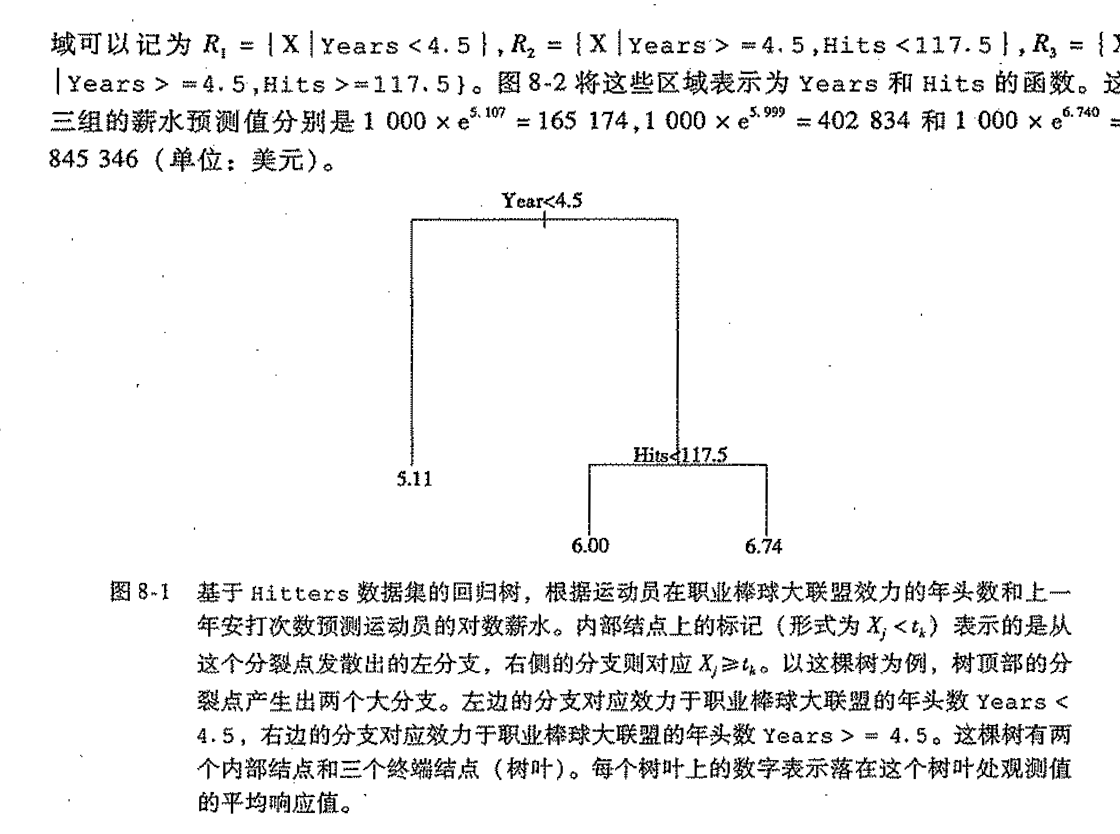
2.10.1. loss function

• Def: loss = RSS

  

2.10.2. optimization

• choose Xj & separate point to make RSS smallest

  

• repeat

  

  

• overall

  

• regularization

  

  

  

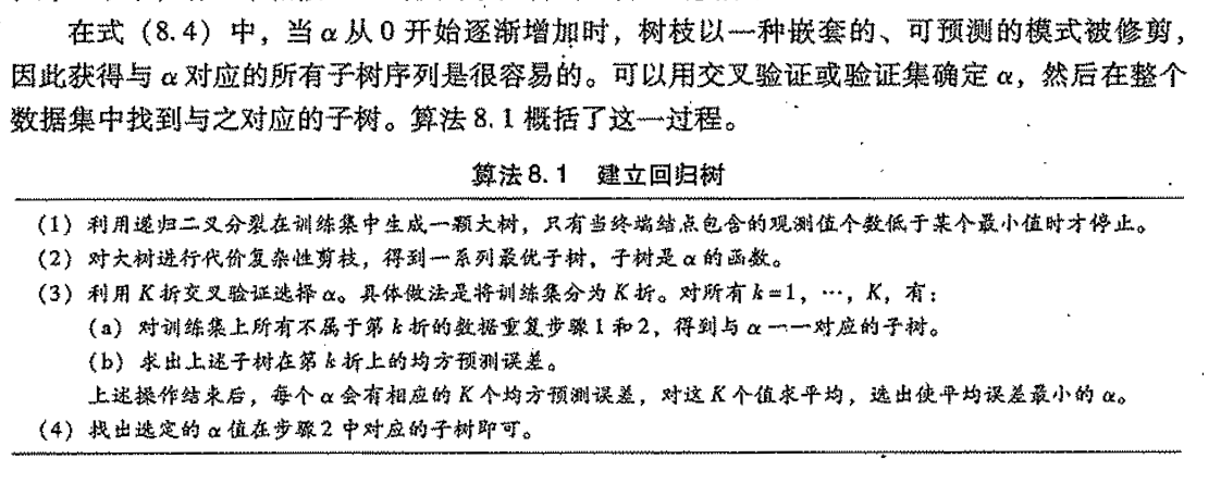
2.11. decision tree

• Usage:

  

• Def: same, only node value = 1/0

2.11.1. loss function

2.11.1.1. error rate

• Def: split into 2 to make loss1+ loss2 small. remember loss1 & loss2 are all in forms below. error ate

  

  • note: how to get f: preset structure: tree model

  • note: how to get res: intuition

  • note: how to get f ha: minimize EmL = loss + weight, by spliting tree.

2.11.1.2. information gain

• Def: entrophy

  

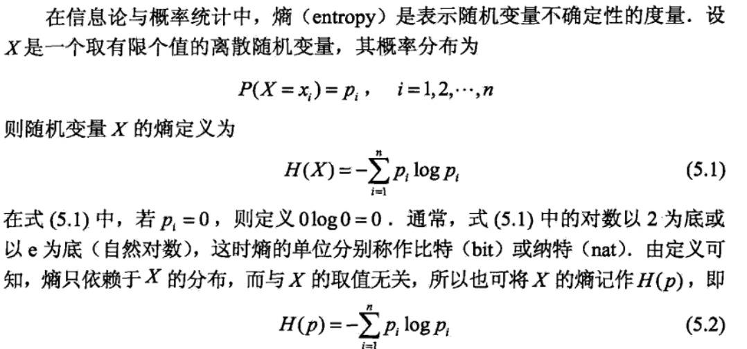
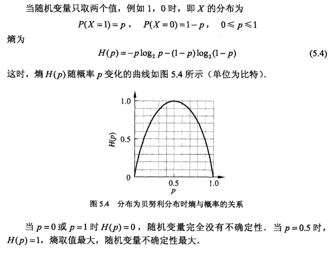
  • Qua:

    

  • Note: example

    

• Def: conditional entrophy

  

• Def: information gain

  

  • Note: choose node with largest information gain (when constrained in A, entrophy drops)

    

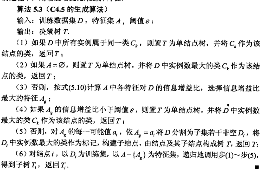
2.11.1.3. information gain ratio

• Def:

  

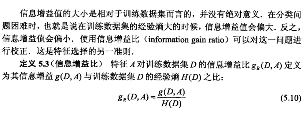
2.11.1.4. gini

• Usage: gini is different from IG, but similar

• Def:

  

  

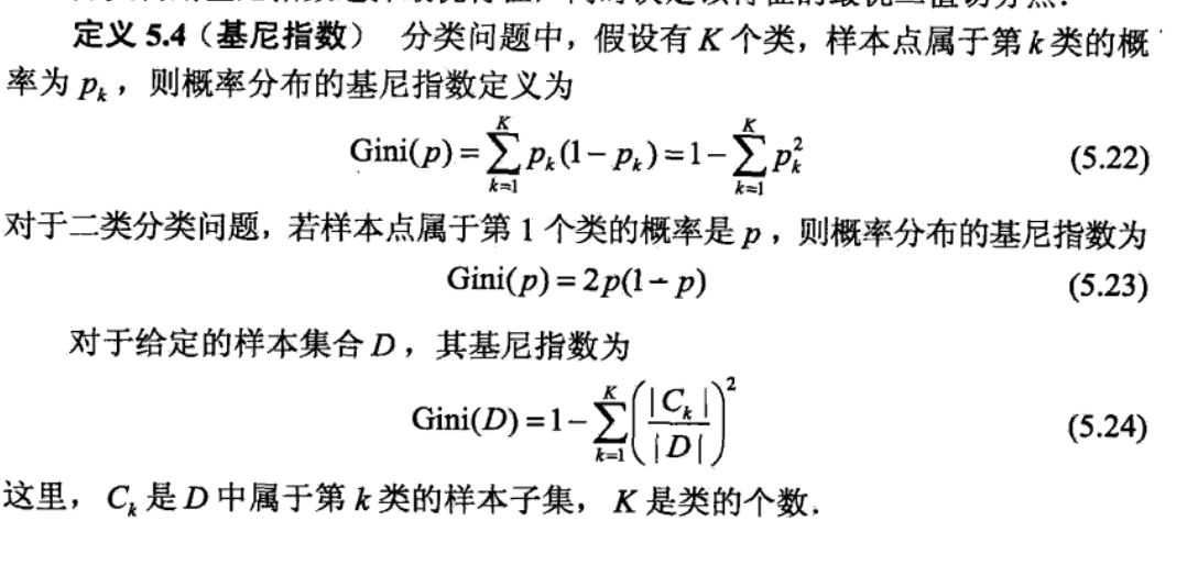
  • Note: the smaller the better

2.11.1.5. cross entrophy (no)

• Def: cross entrophy

  

  • Usage: since entropy is a constant, we only need to minimize cross entrophy

• Def: KL = cross - entropy

  

  • Usage: to determine differences between distributions

2.11.2. implementation

2.11.2.1. ID3

• Usage:

  

• Def:

  

  

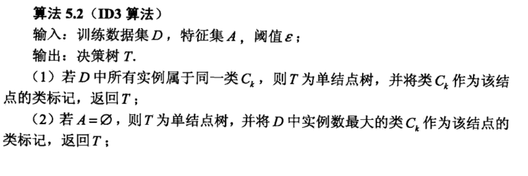
  • Note: that each path contains no duplicate features.

2.11.2.2. C4.5

• Usage:

  

• Def:

  

2.11.2.3. CART

• Usage: binary tree!!

  

• Def:

  

  

2.11.3. alternatives & improvement

2.11.3.1. trimming

• Usage: overfitting

  

  

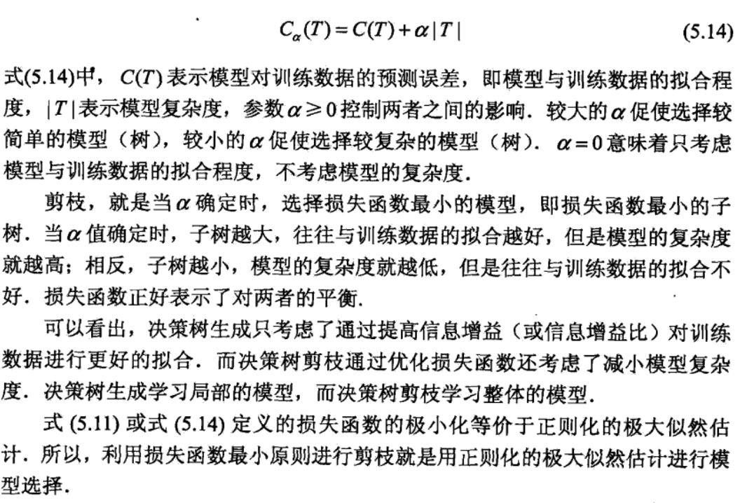
• Def:

  

  

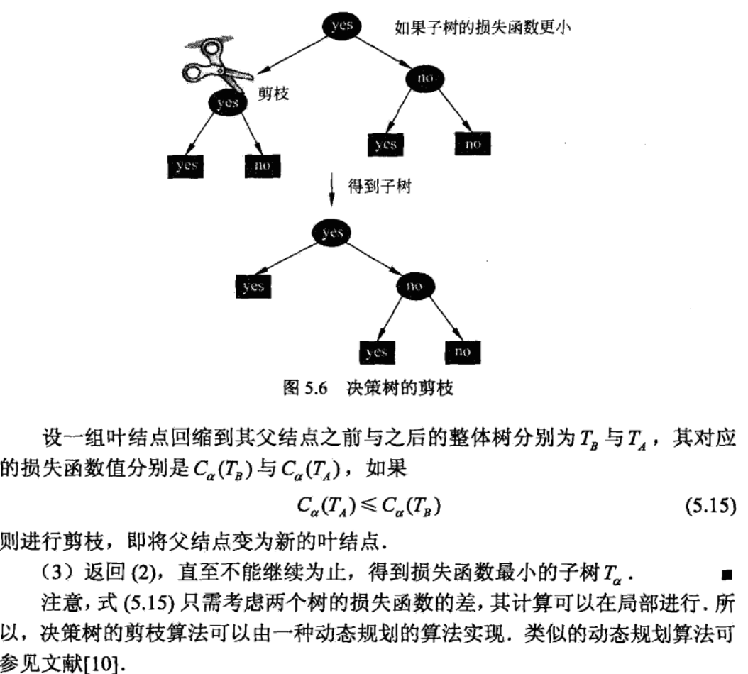
  • Note: start from all leaves, and trim children if tree+chidren cost more than tree, this is likely since |T| is in loss function.

2.11.3.2. bagging tree

• Def:

  

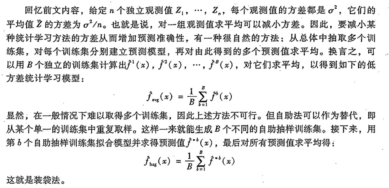
2.11.3.3. random forest

• Def:

  

  

  • Qua: difference with baggin

    

2.11.3.4. boosting

2.12. dnn algorithm

2.12.1. regularization

3. unsupervised algorithms

3.1. clustering analysis

• Usage: given => data(X1,X2,...XN), output=>(X1,cluster)...(XN,cluster)

3.1.1. transformation

• Def:

  

  img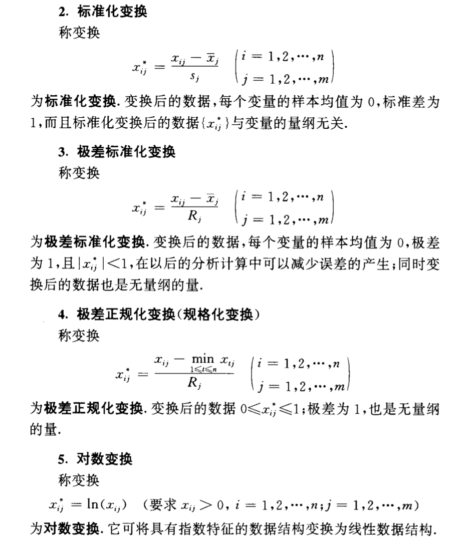

  

  img

3.1.2. distances

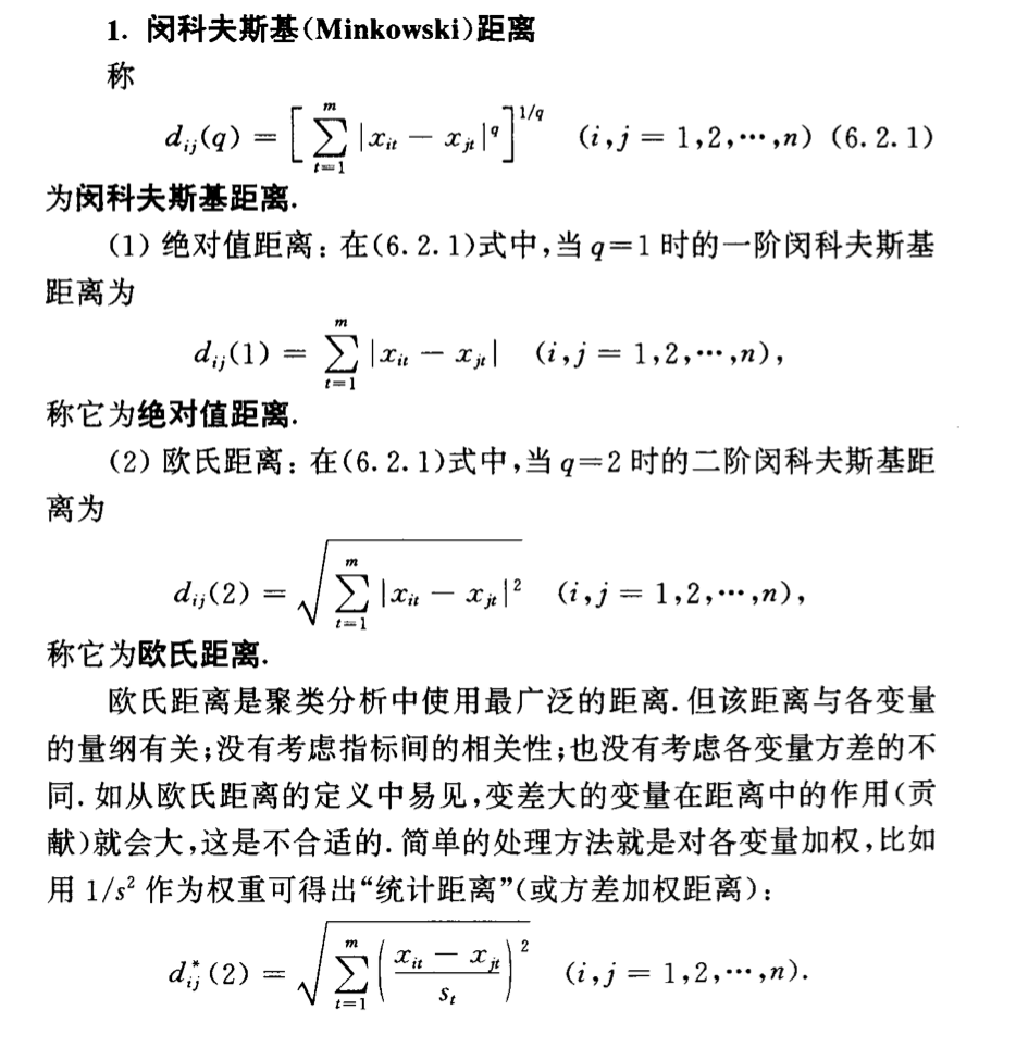
3.1.2.1. between samples

• Def:

  

  img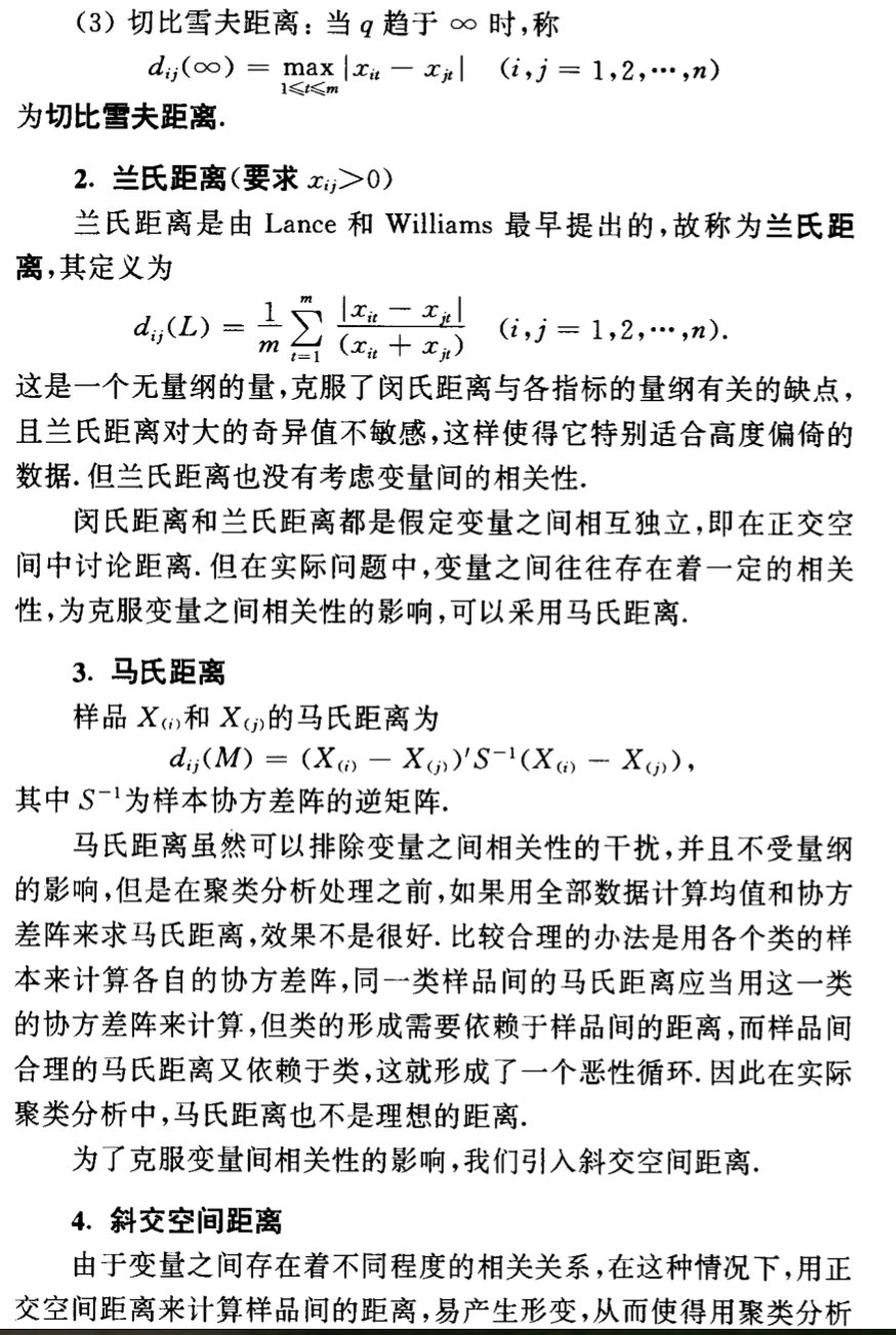

  

  img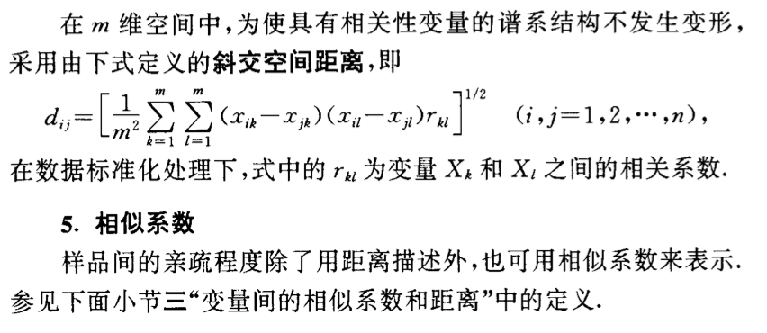

  

  img

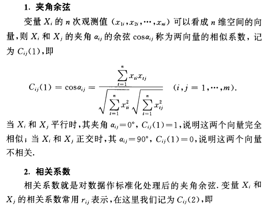
3.1.2.2. between features

• Def:

  

  img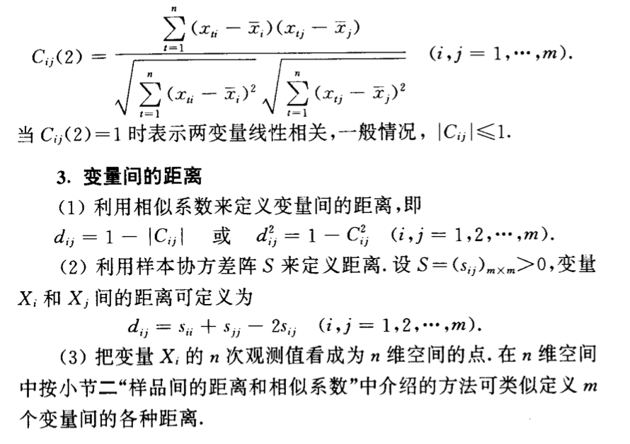

  

  img

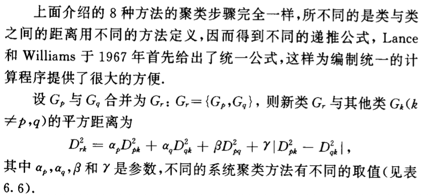
3.1.2.3. between clusters

• Def:

  

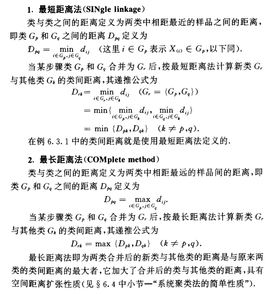
  img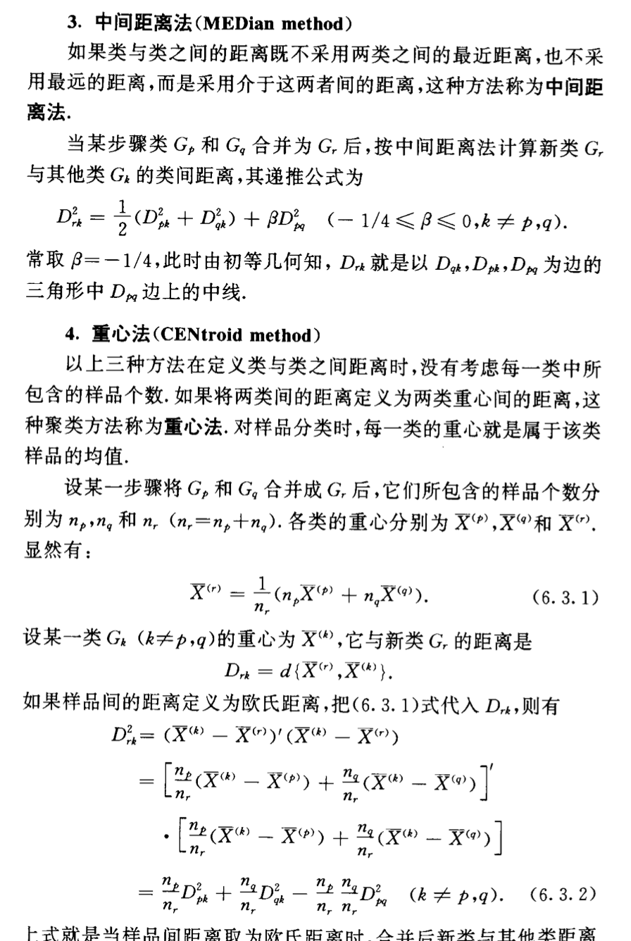

  

  img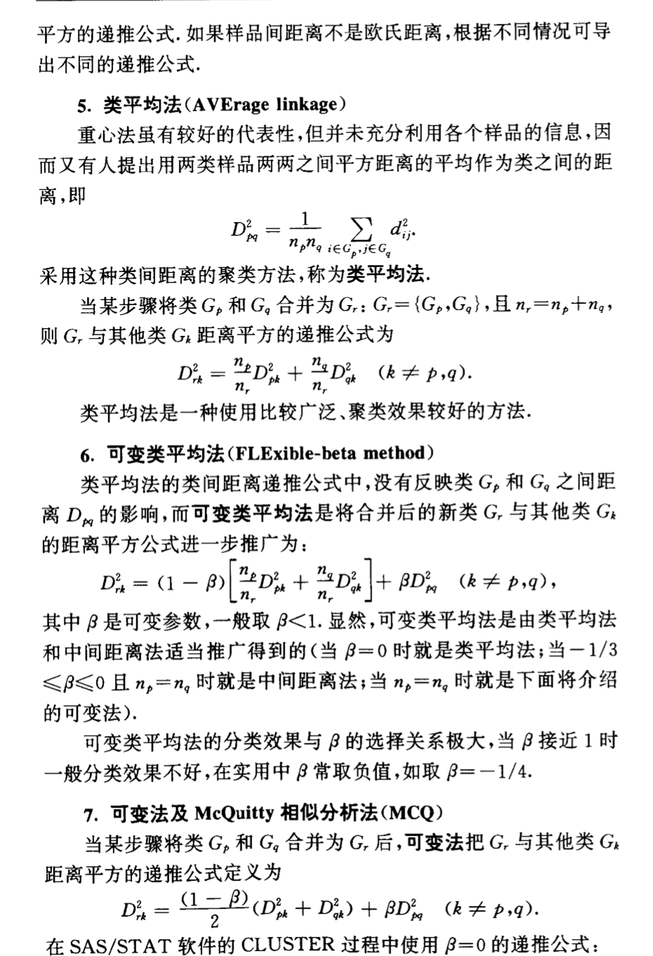

  

  img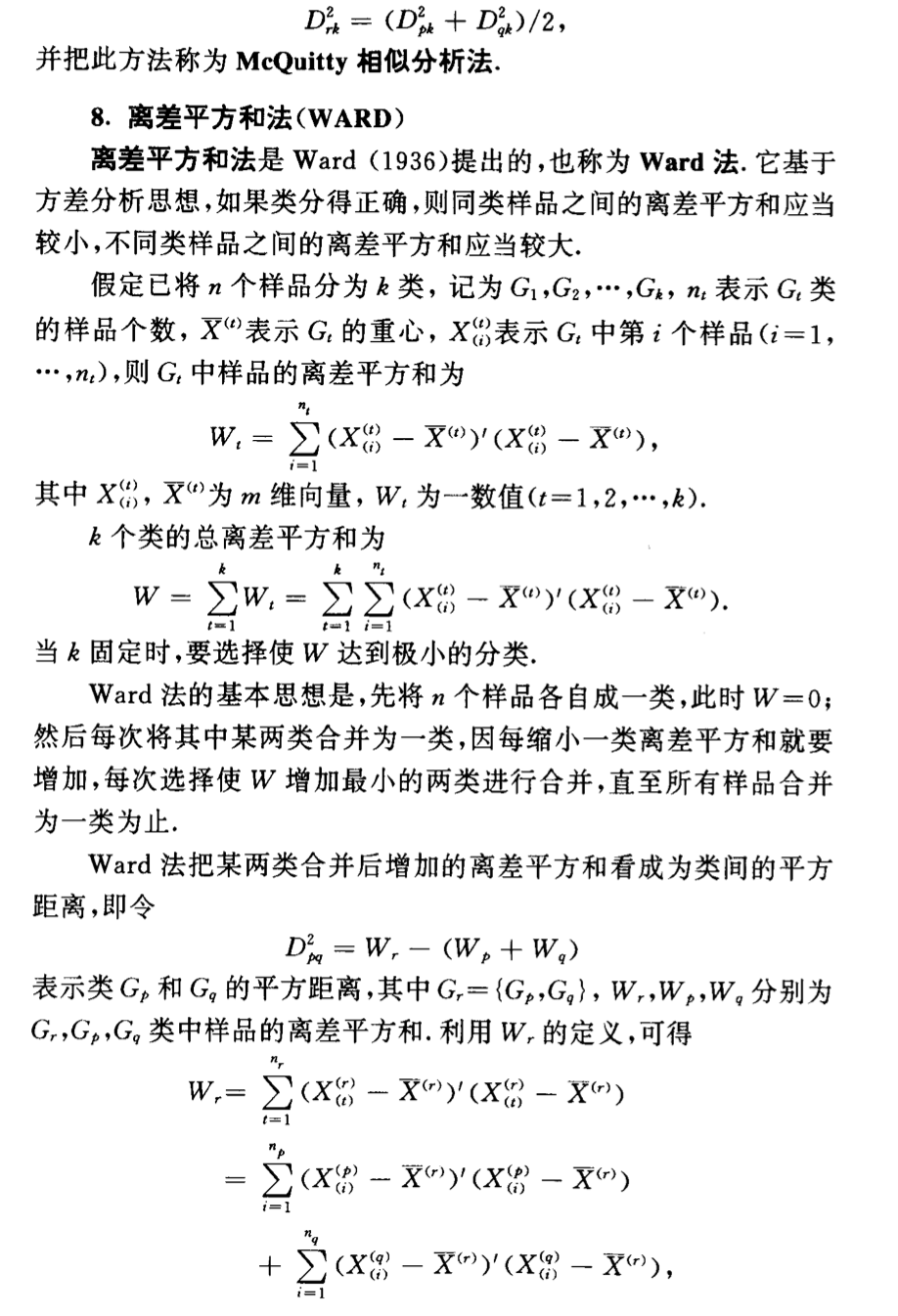

  

  img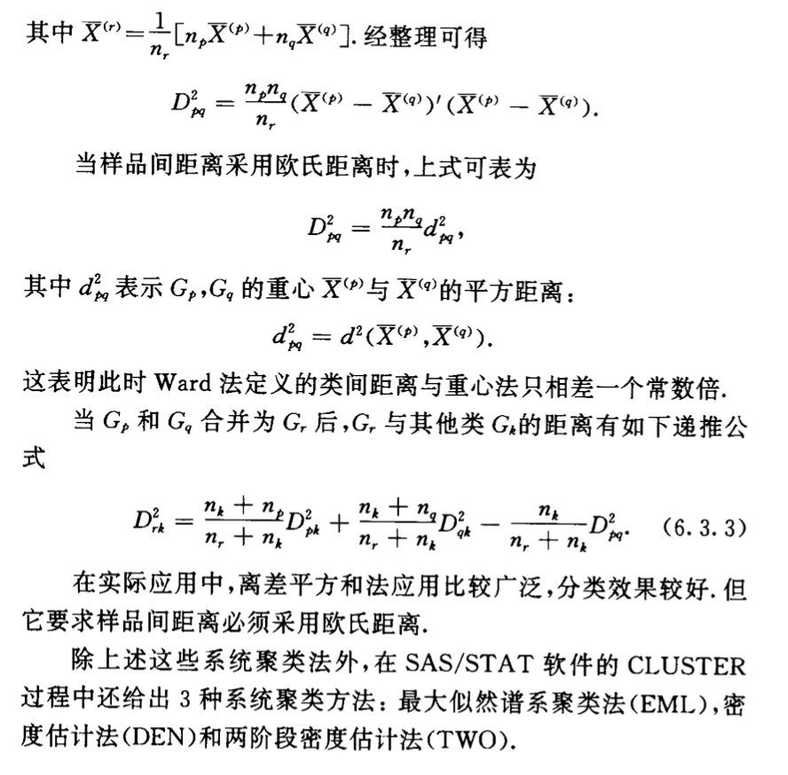

  

  img

• Theorem: overall:

  

  img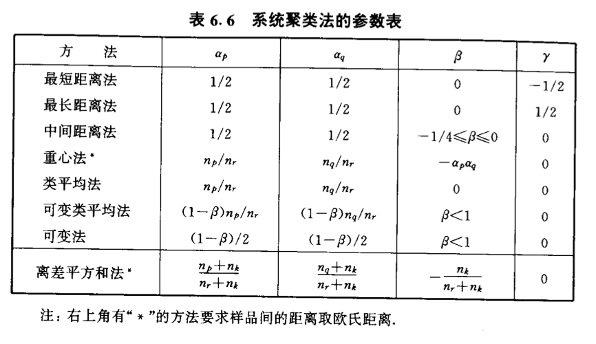

  

  img

3.1.3. hierarchical clustering

• Algorithm:

  

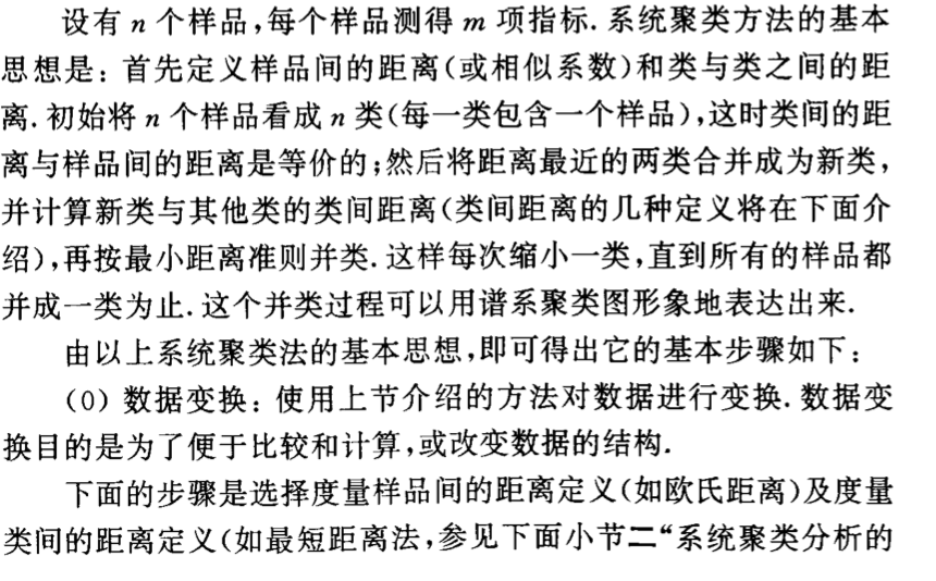
  img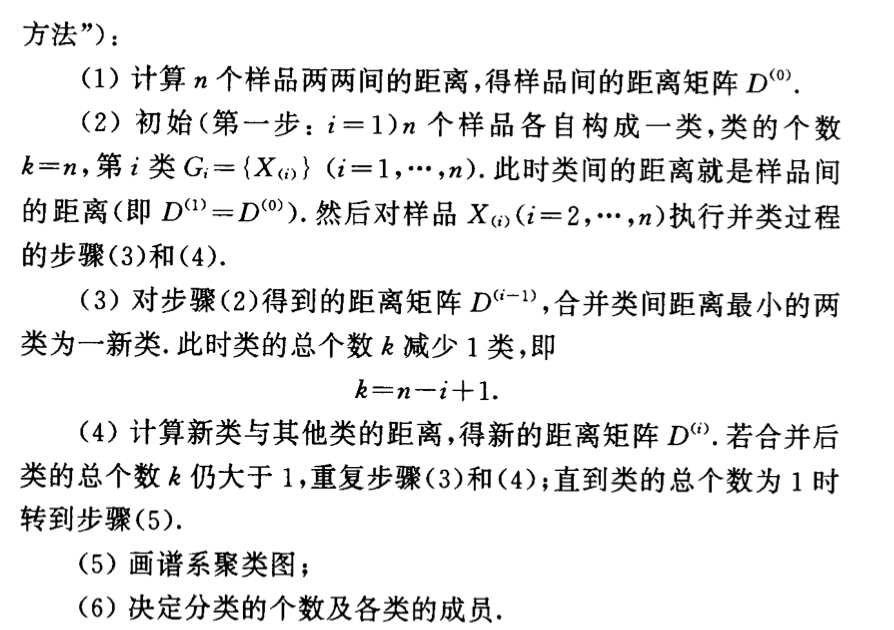

  

  img

  • Qua: => distance are mono

    

    img

  • Qua: => s

    

    img

• Qua: how to set the cluster number

  P245

3.1.4. dynamic clustering

3.1.4.1. batch wise

• Algorithm:

  

  img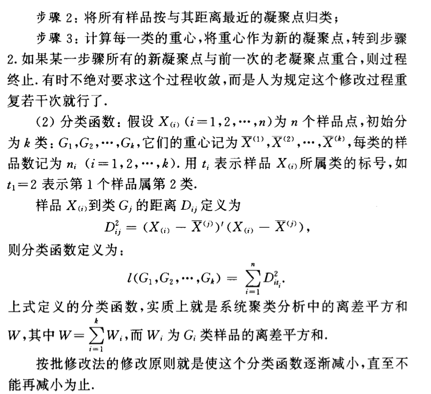

  

  img

3.1.4.2. sample wise(kmeans)

• Algorithm:

  

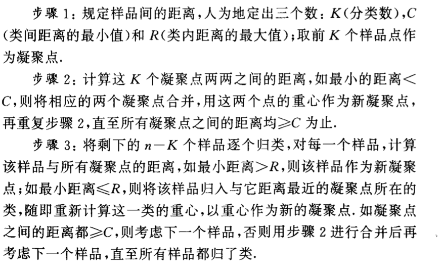
  img

  

  img

3.2. principal component analysis

3.2.1. PCA

• Usage: given data(X1...XN), output datalessdimension(X'1...X'N)

• Def: principle vector

  

  img

  Note:

  

  img

  • Qua: ways to compute

    

    img

    

    img

    

    img

  • Qua:

    

    img

• Def: 因子负荷

  

  img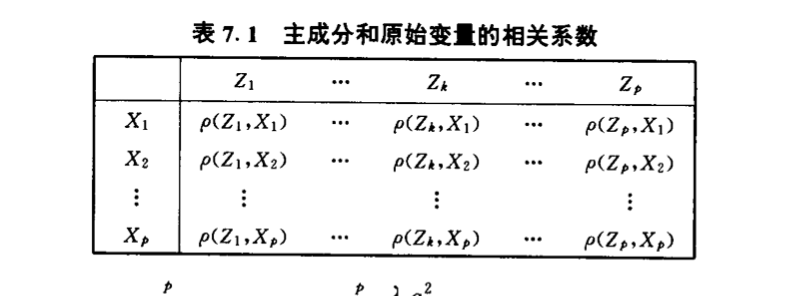

  

  img

  • Qua:

    

    img

• Qua：

  

  img

• Def: total variance

  

  img

• Def: contribution

  

  img

• Def: contribution2

  

  img

3.2.2. standardized PCA

• Def:

  

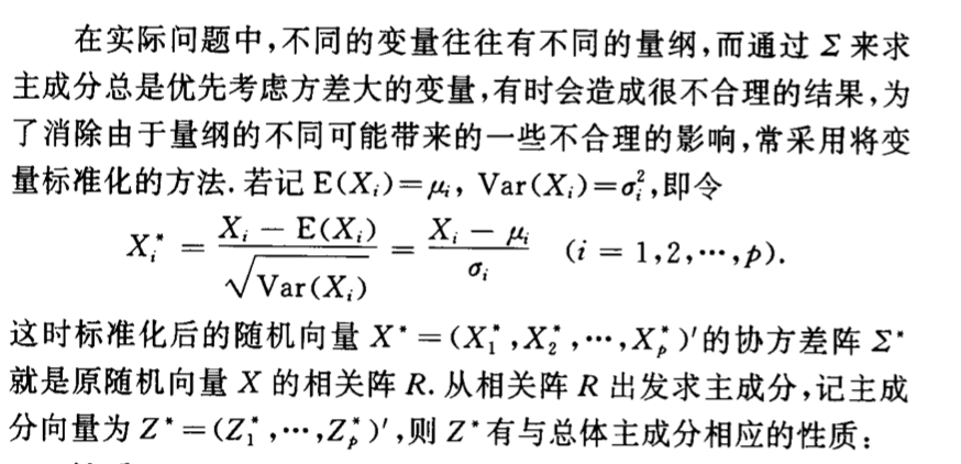
  img

  • Qua:

    

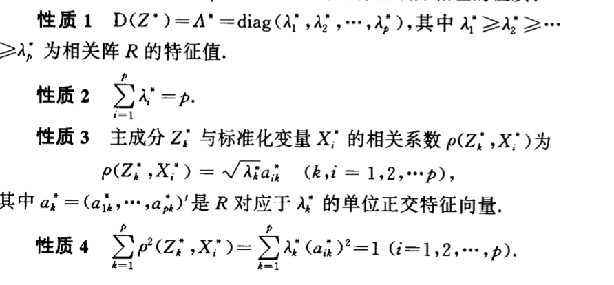
    img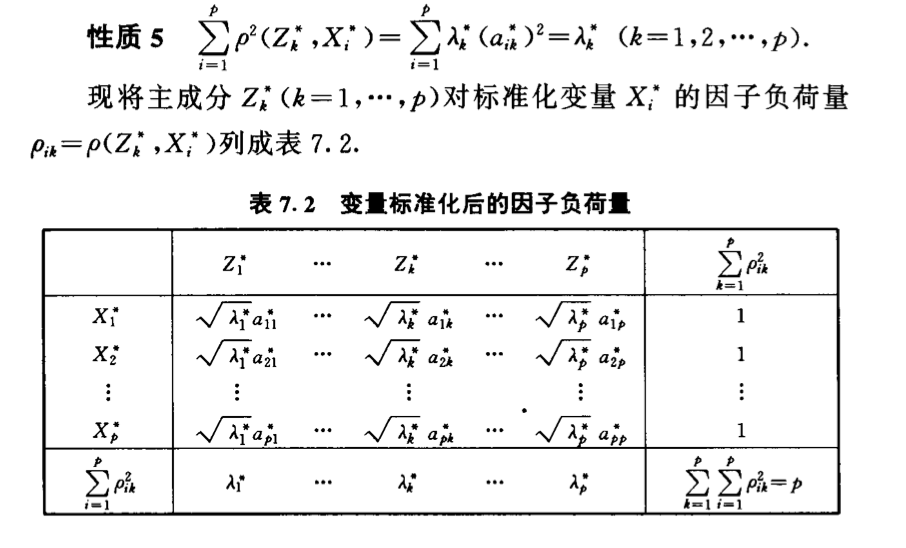

    

    img

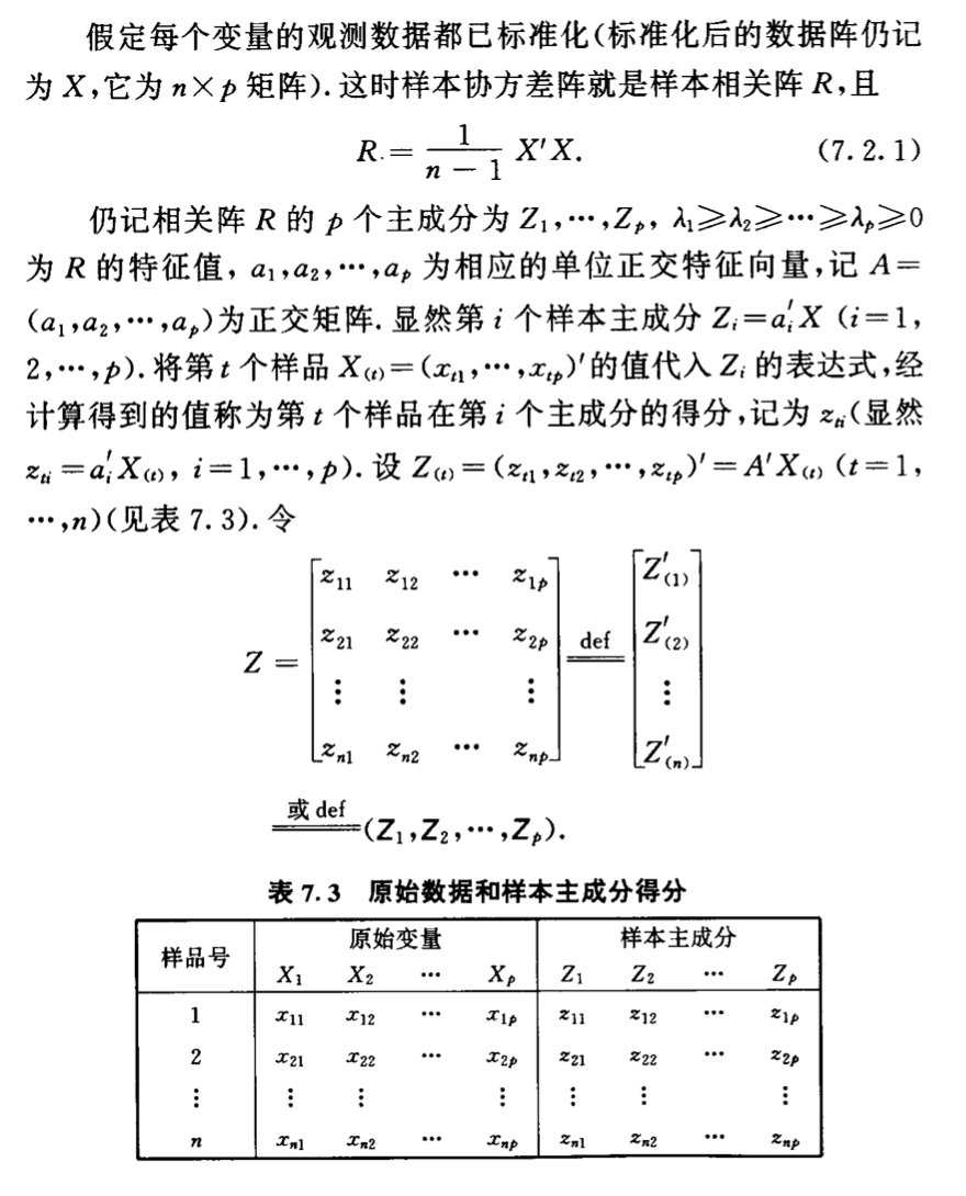
3.2.3. sample PCA

• Def:

  

  img

  

  img

  • Qua:

    

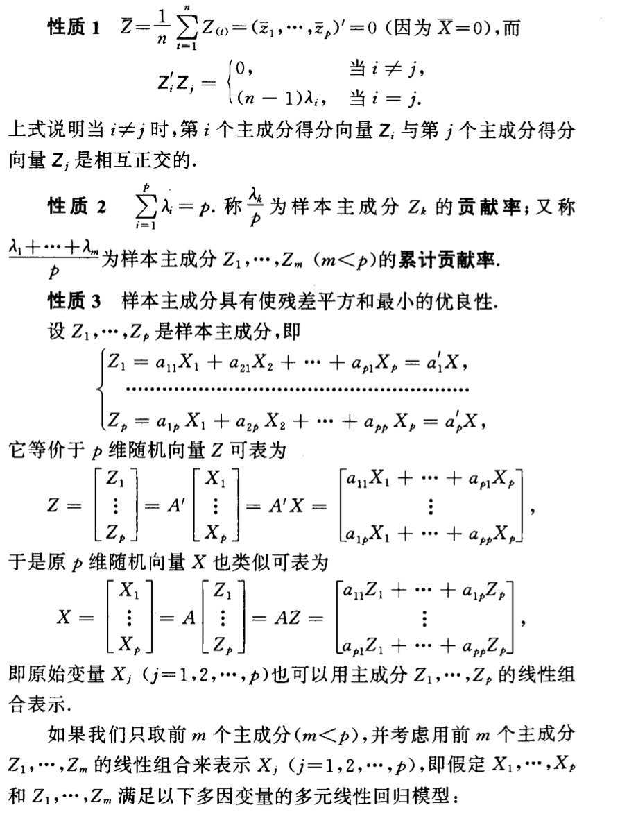
    img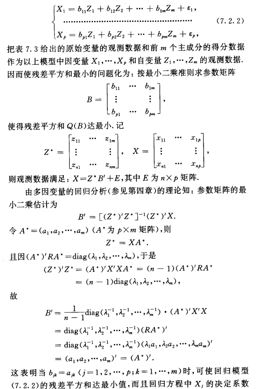

    

    img

    

    img

3.3. factor analysis

3.4. canonical correlation analysis

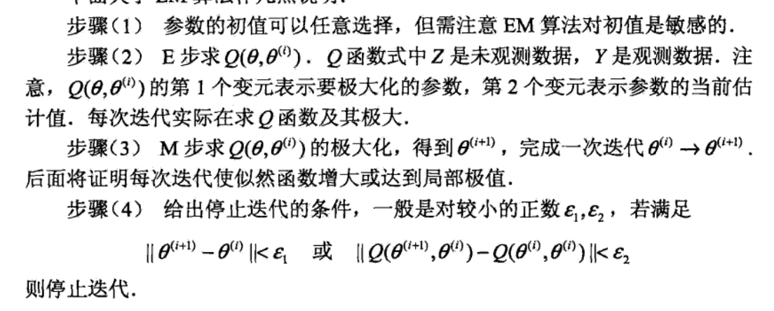
3.5. EM

• Usage: input => data(X1,X2,...Xn), output => parameters concerning X's distribution, a step-wise & approximate algorithm of max likelihood.

  

  img

  why can't use max likelihood? because it contains log of sum => hard to get derivative. Note that z does not appear on the left, it means that we can not observe z or other wise we can put \(p(y,z |\theta )\) together and get \(p(y,z|\theta)=p(z|\theta)p(y|z,\theta)=\pi ^{z}(1-\pi) ^{1-z}p^{yz} (1-p) ^{(1-y)z}q ^{y(1-z)}(1-q) ^{(1-y)(1-z)}=(\pi p ^{y}(1-p) ^{1-y}) ^{z}...\), this is very easy to estimate via max likelihood. The general idea is that with more data, the problem will become more easy to solve.

  

  example of using EM algorithm

  

• Def: Q function

  

• Def: EM, hardest part is to get Q.

  

  • Note: some notices,

    

3.5.1. loss function

• Def: max likelihood . This is the function we wish to maximize

  

  this is the function we actually maximize

  

  • Note: f comes from preset model with parameters (e.g. normal distribution)
  • Note: \(\hat{f}\) comes from step-wise optimization with data.

3.5.2. optimization

• Def: we want to use step-wise optimization

  

  getting lower bound for the differentiate by Jensen

  

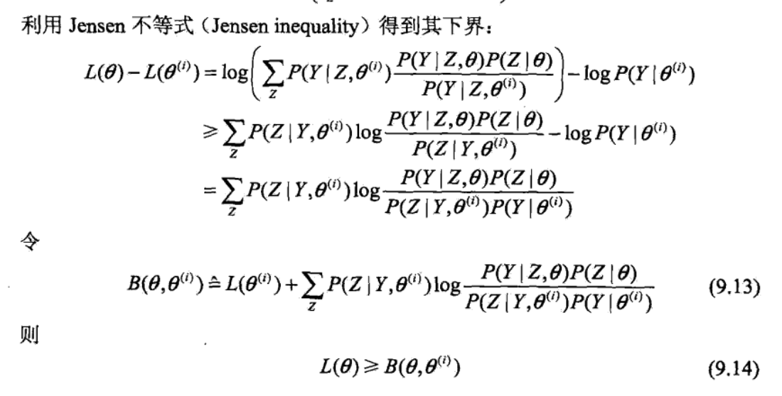
  using lower bound to do step-wise optimization

  

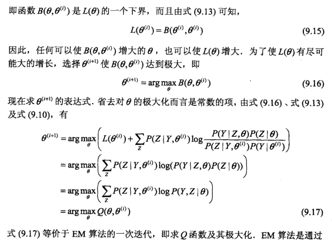
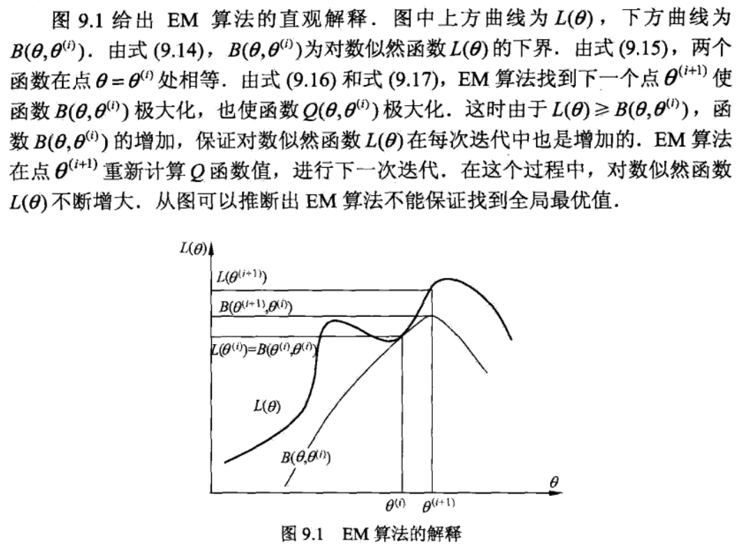
  • Note: illustration very good => in each round, we maximize \(B(\theta, \theta_i)\) to get \(\theta_{i+1}\), then we get \(B(\theta, \theta_{i+1} )\) which is another lower bound curve and we seek for peak for that. this is a non-decreasing algorithm since B is lower bound and we always seek peaks on B.

    

3.5.3. convergence

• Theorem:

  

• Theorem:

  

  • Note:

    

3.5.4. alternatives & improvements

3.5.4.1. GMM

• Def: GMM

  

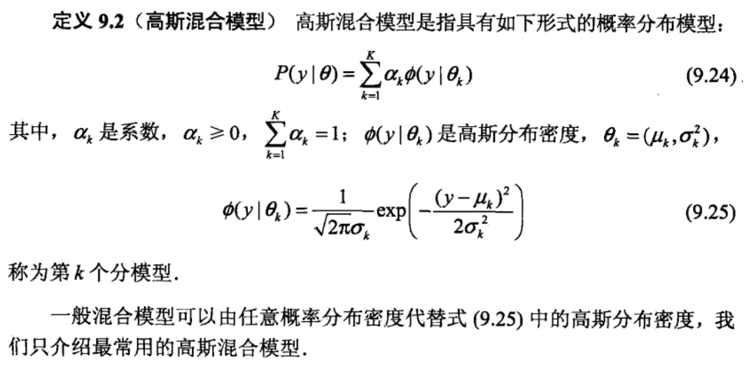
  first we need to know what parameters to estimate, what hidden variables we don't know. Note that we can make up a hidden variable so that the post probability is the same => we can image we first choose randomly from 1->k and then generate result. The max likelihood function can be computed by full probability expansion/

  

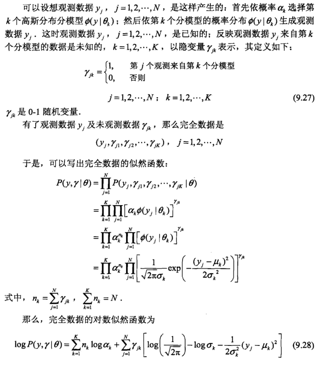
  define Q

  

  expand Q

  

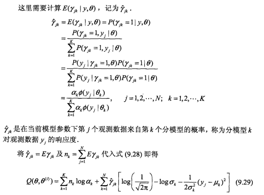
  maximize Q

  

  

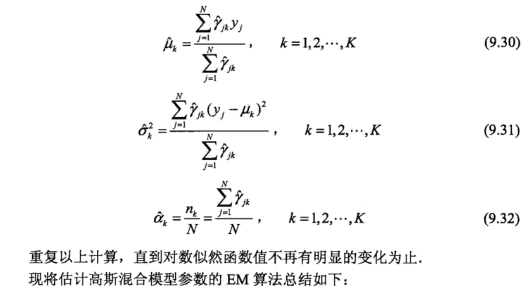
  overall

  

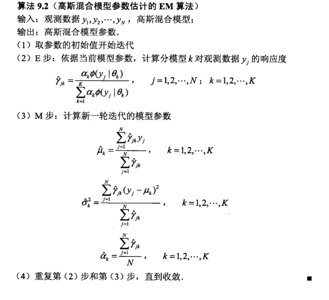
3.6. markov algorithm

4. reinforced algorithms

lecture 2基本介绍了基本前置定理比如vc之类的；

lecture 1先是介绍了基本算法等，然后用average和hoeffding bound介绍了EPM思想。

lecture 3先是介绍了基本框架，然后用EPT证明各种bound，然用用这些bound介绍EPM思想。