Regression Analysis Course Slides Notes
1. regression methods
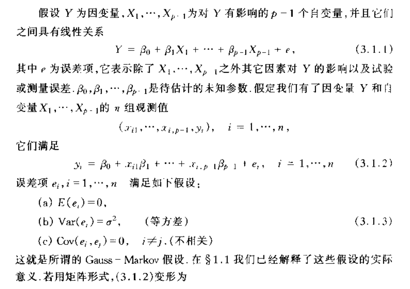
1.1. basic hypothesis
Def: Gaussian Markov Condition
1.2. basic least square
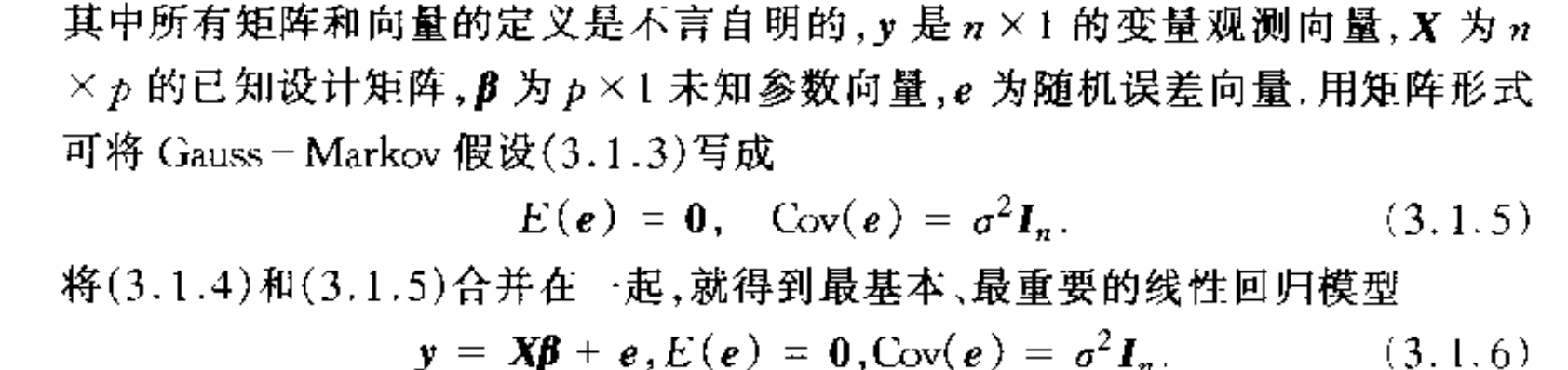
Def: basic linear model
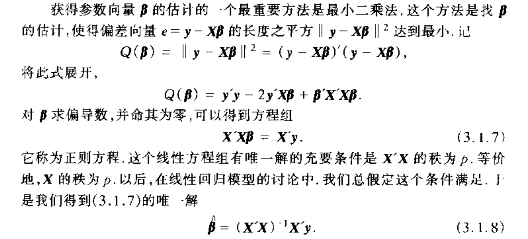
Algorithm: least square
1.2.1. expectation & var
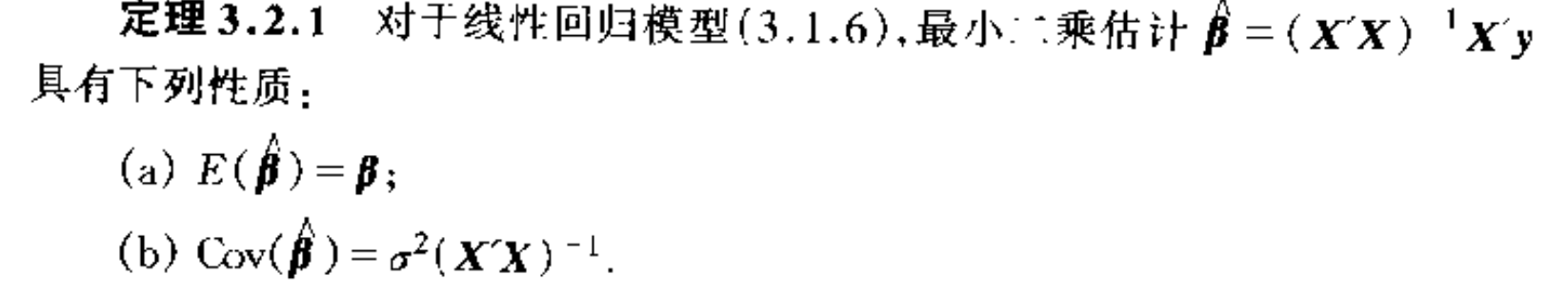
Qua: => expectation & var of least square
Theorem: => for all the linear unbiased, least square has least var


Note:
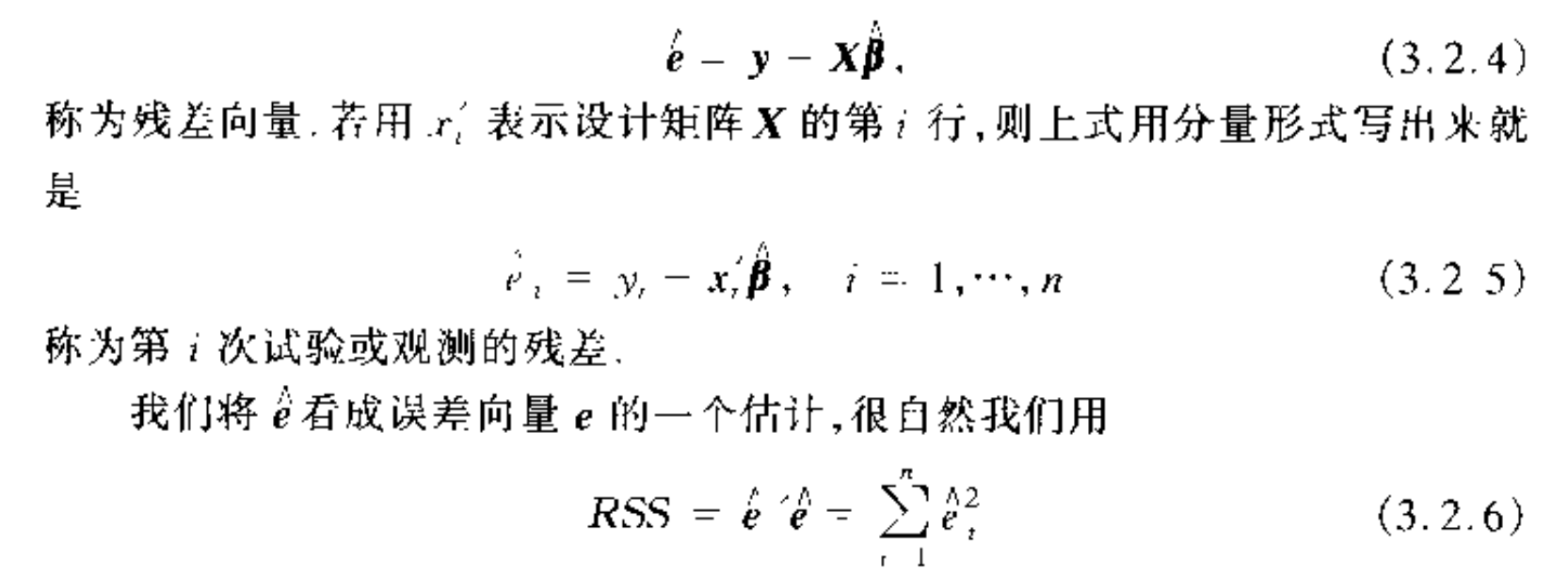
1.2.2. residual sum of squares ( RSS )
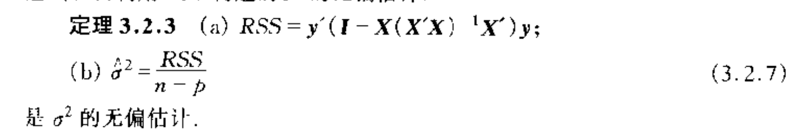
Def: RSS
Note:
Qua: => expectation of residual vector
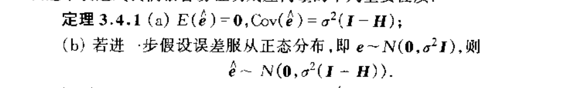
Qua; => expectation of RSS
Qua: => generalized RSS
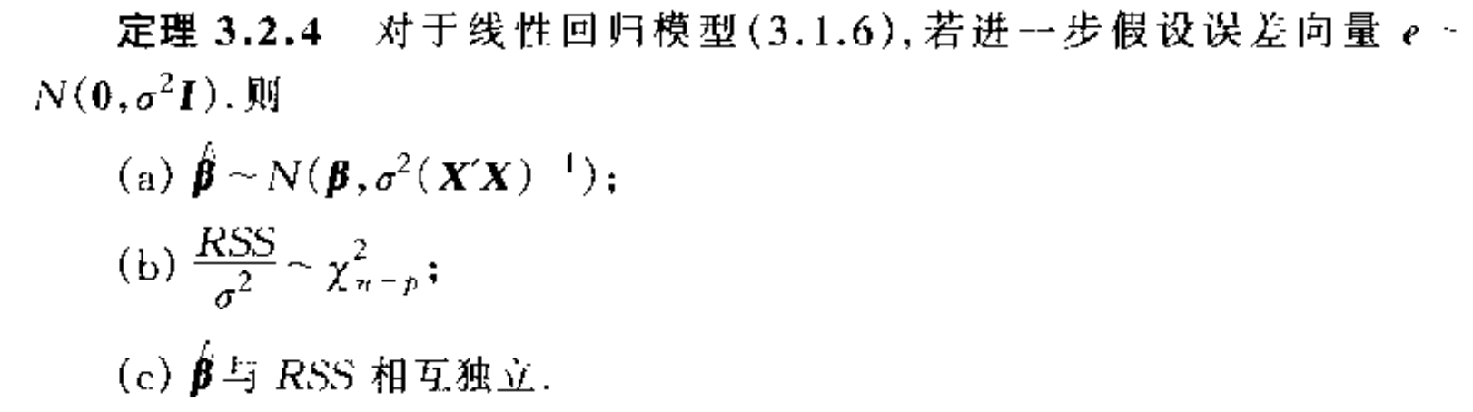
Theorem: => important of RSS (independency is the most important when we do hypothesis test)
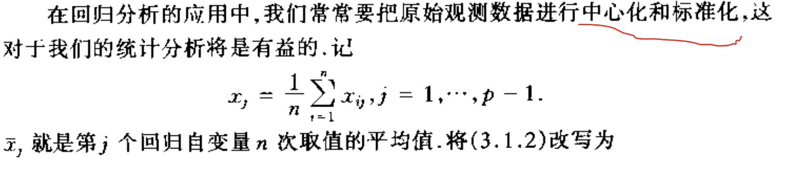
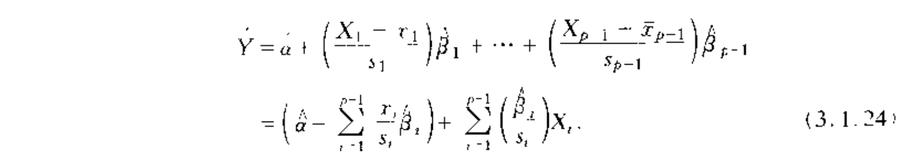
1.3. centralized least square
Def: centralized linear model
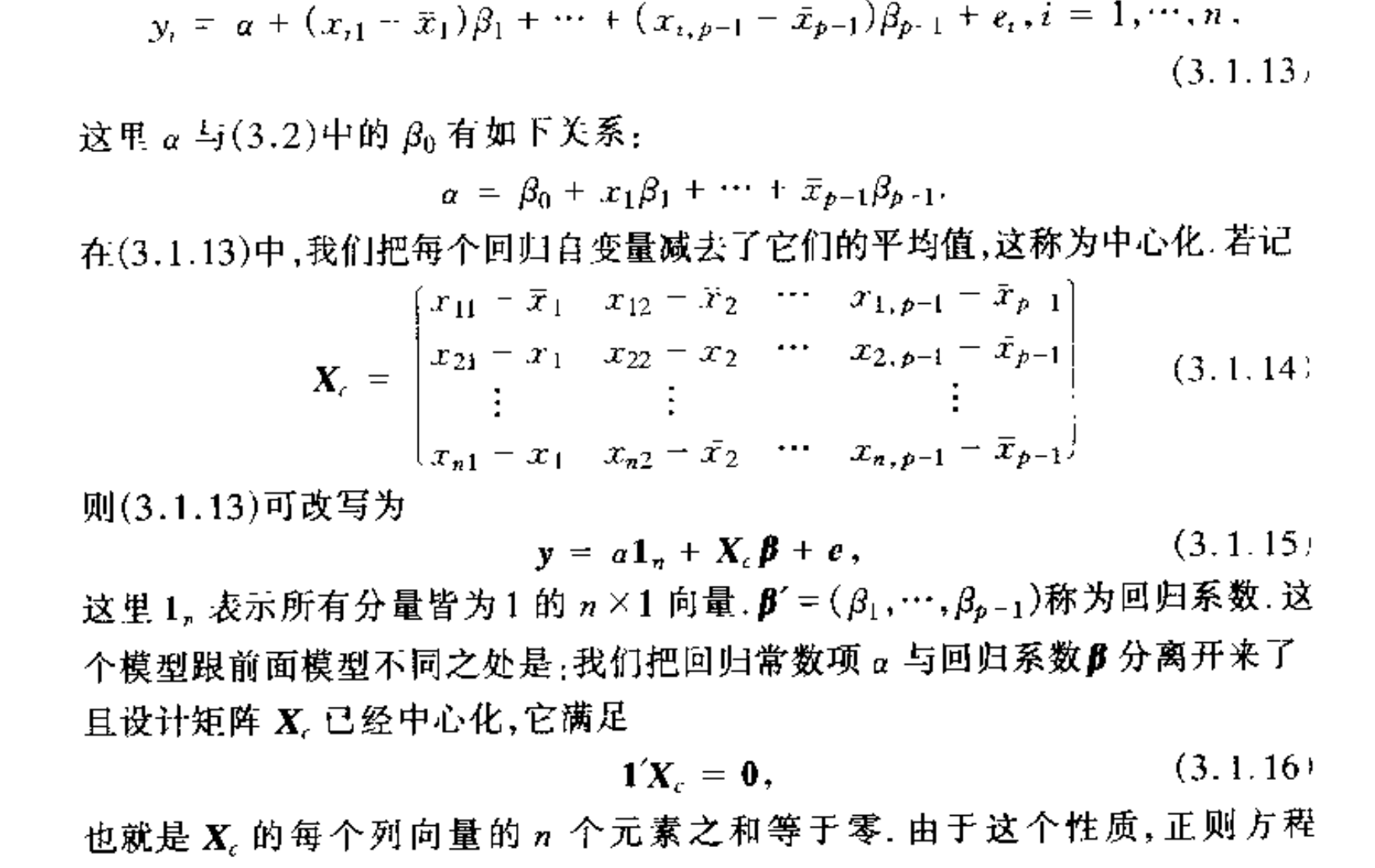
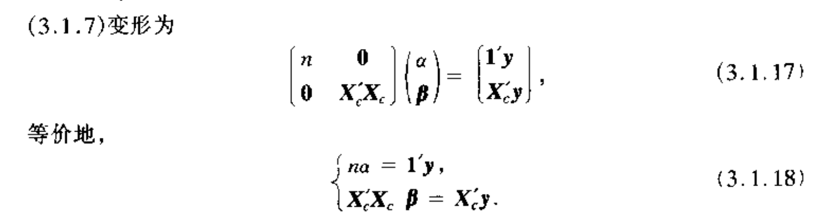
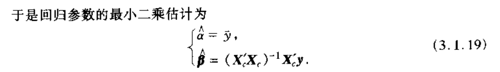
Algorithm: centralized least square
Note:
1.3.1. expectation & var
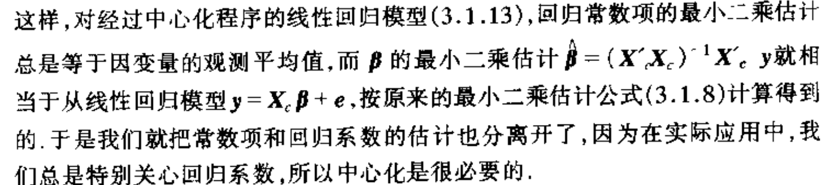
Qua: => expectation
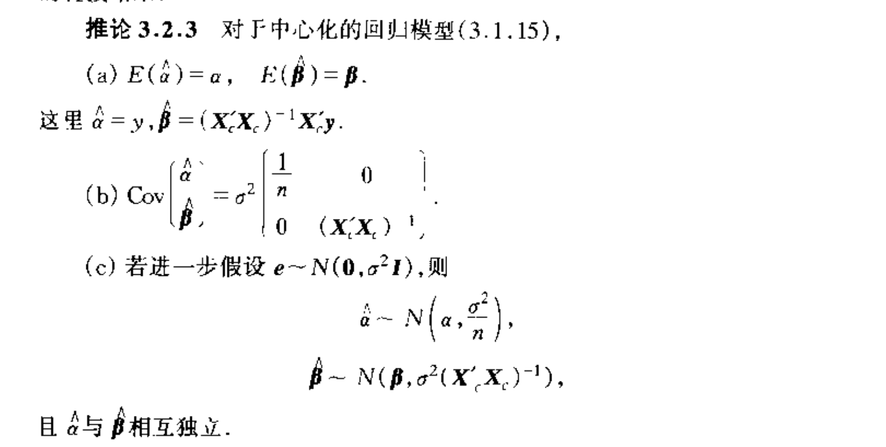
Note: more about centralization
Def: regression coefficient
1.3.2. MSE
Def: see probability theory
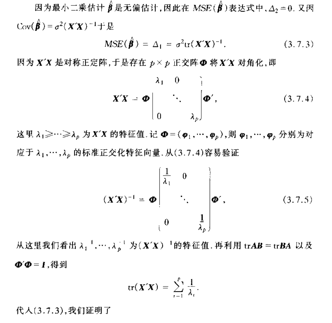
Qua: => MSE of centralized least square

Proof:
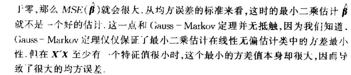
Note: if eigvalue small, then MSE large!
## standardized least square
Def: standardized linear model
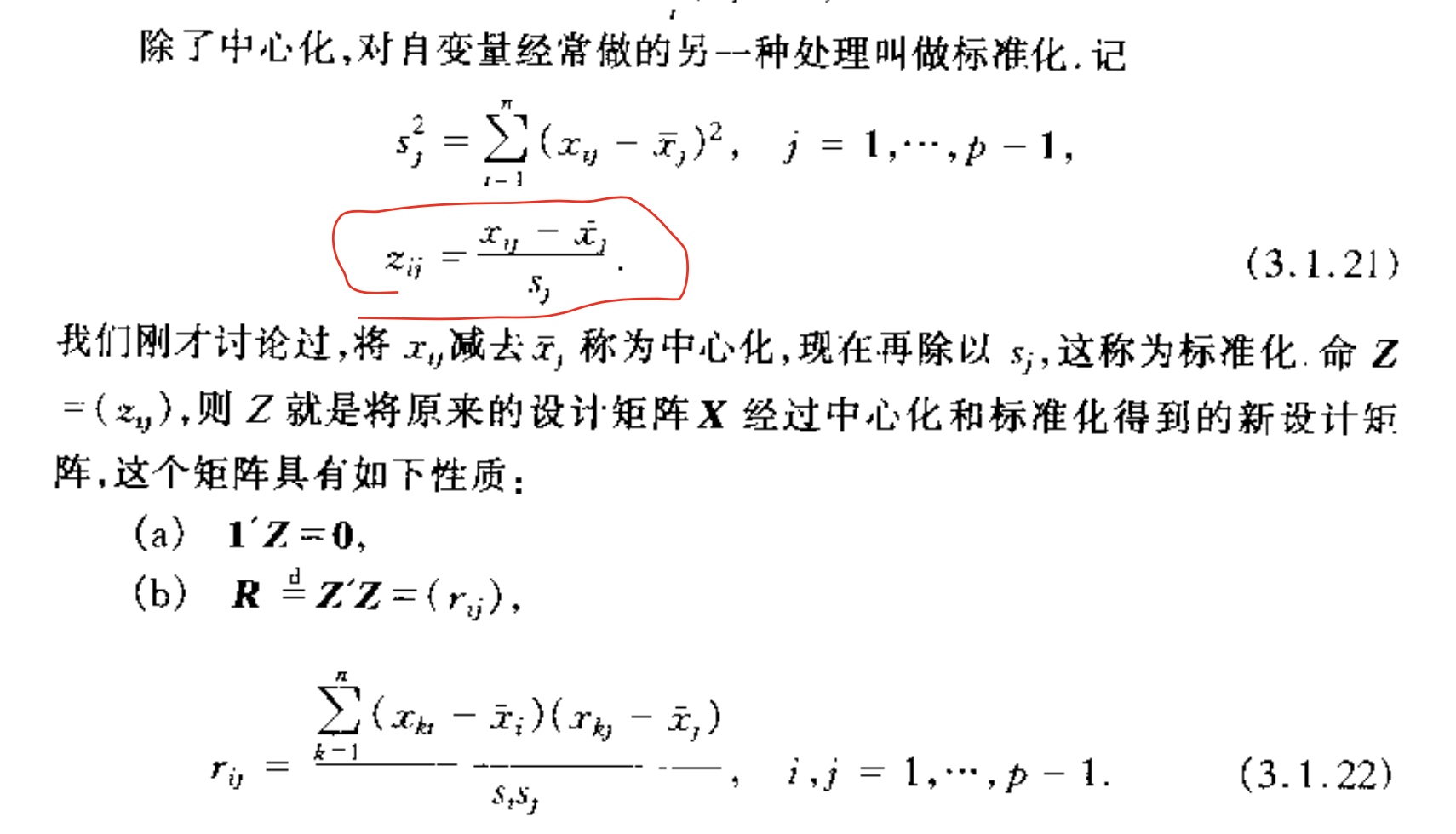
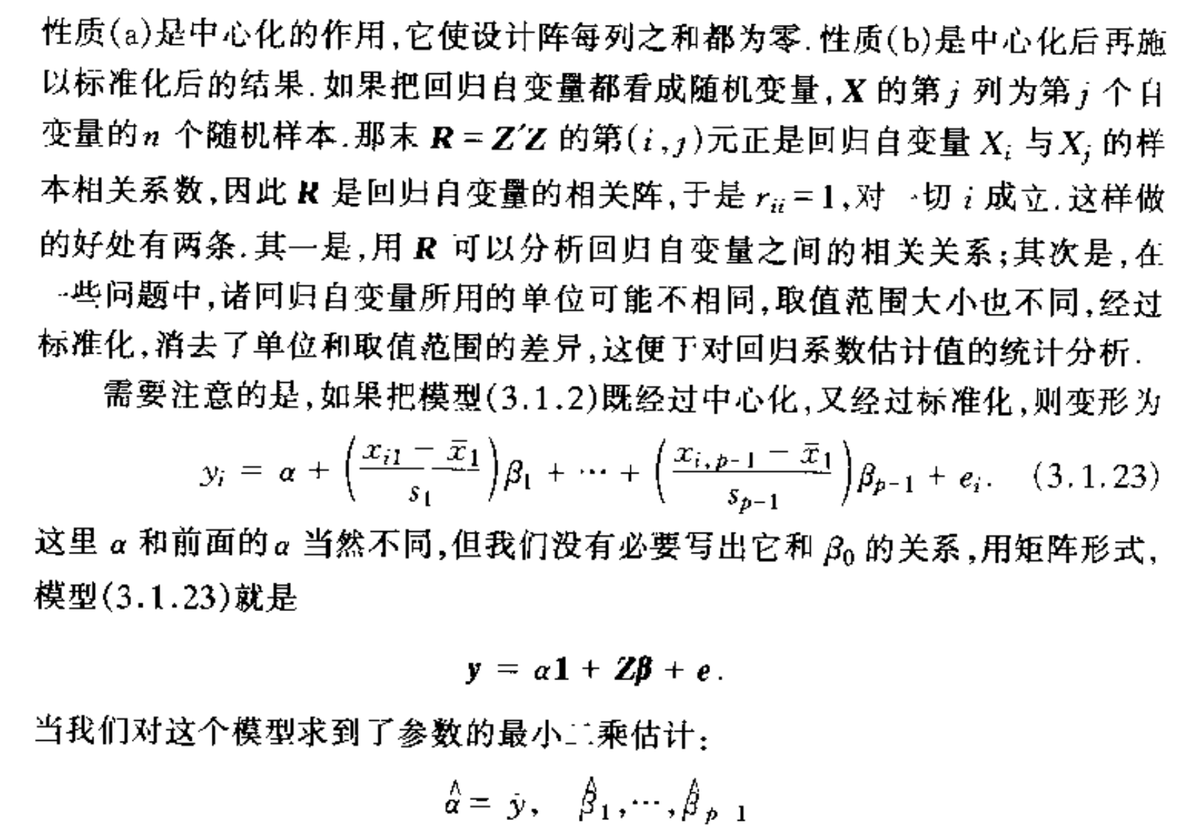
Note: relationship bewteen standardized model and general model.
1.4. constraint least square
Def: contraint linear model
Usage: same model but an additional constraint equation
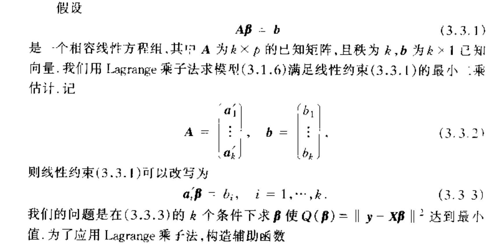
Algorithm: constrainde least square
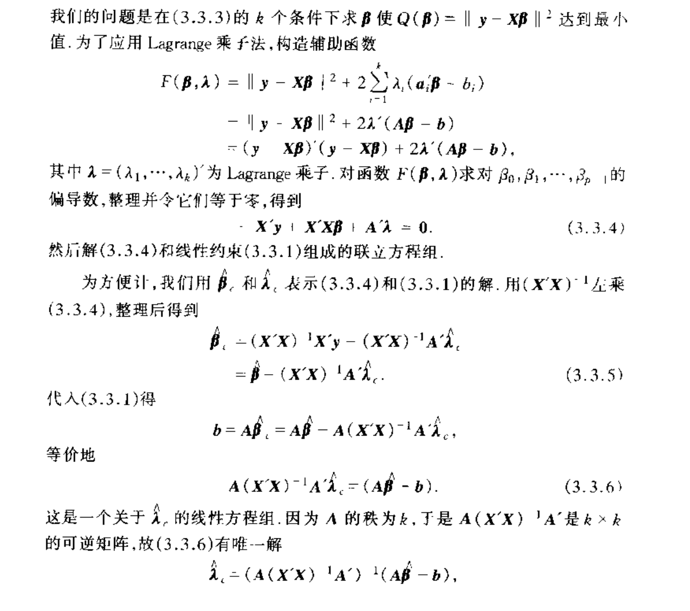
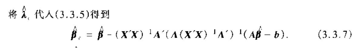
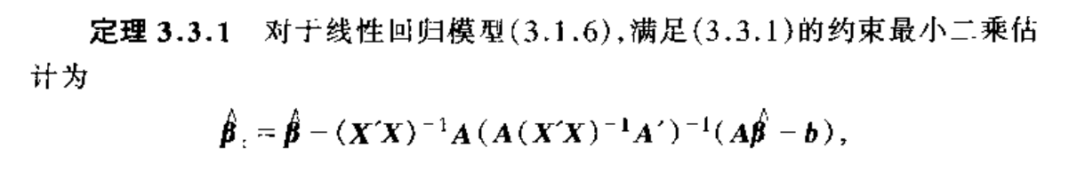
Proof: prove that the min point does exists
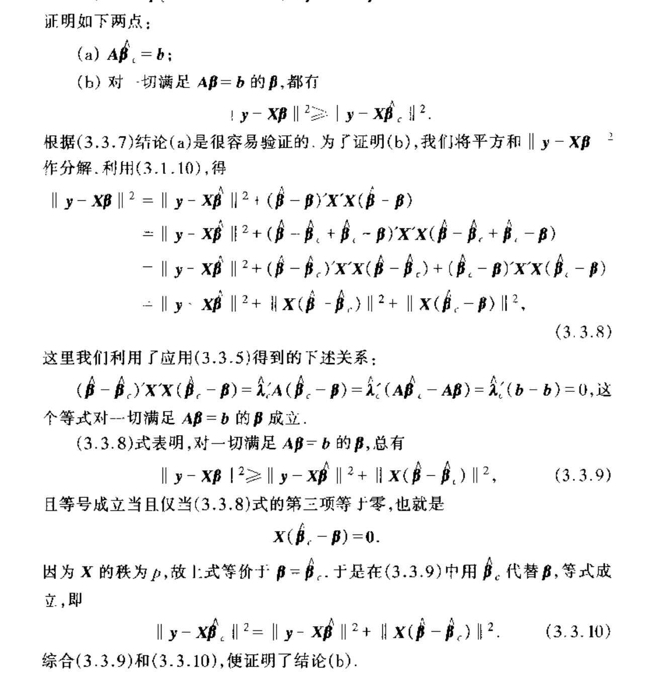
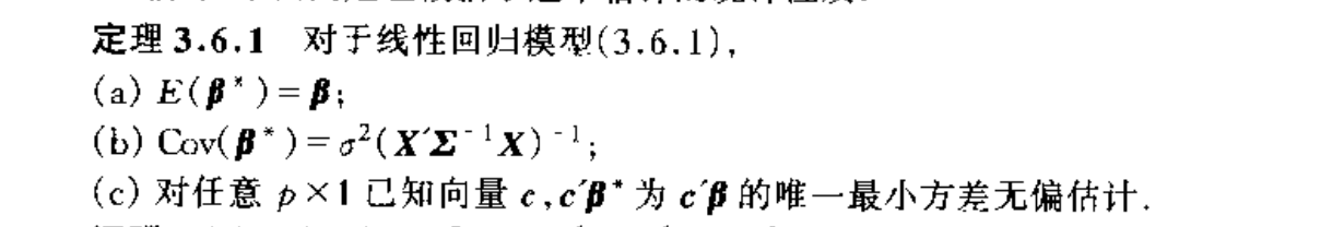
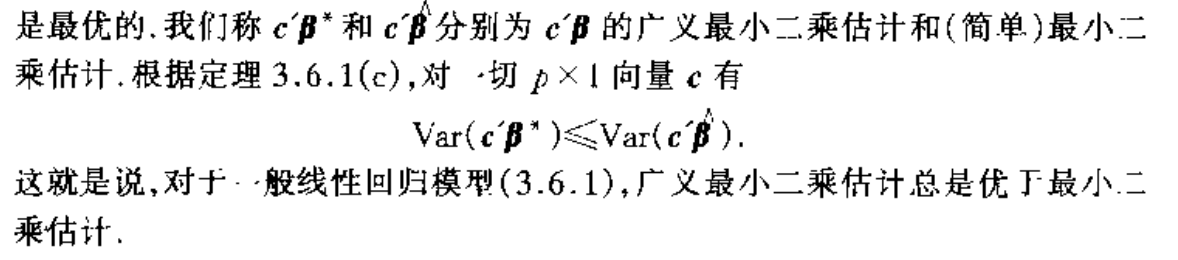
1.5. generalized least square
Def: generalized linear model
Usage: model where covariance matrix is not identical but orthogonal matrix
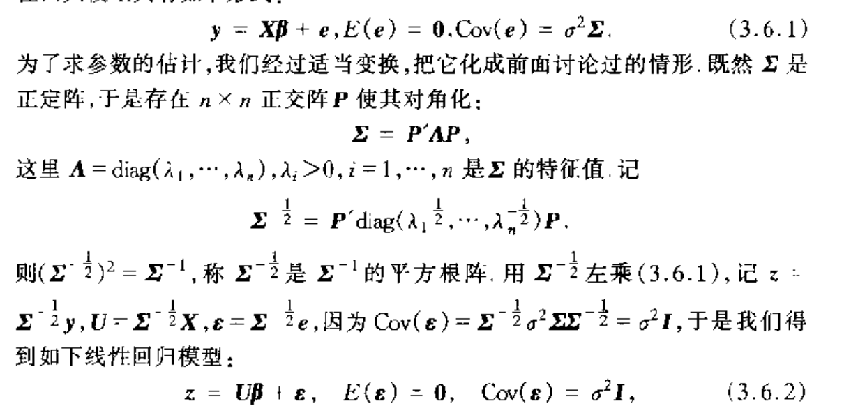
Algorithm: generalized least square

Qua: => expectations
Note: apparently generalized model turn a random model to its standardized form, and it become the best via Gaussain-Markov condition
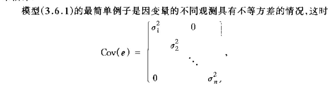
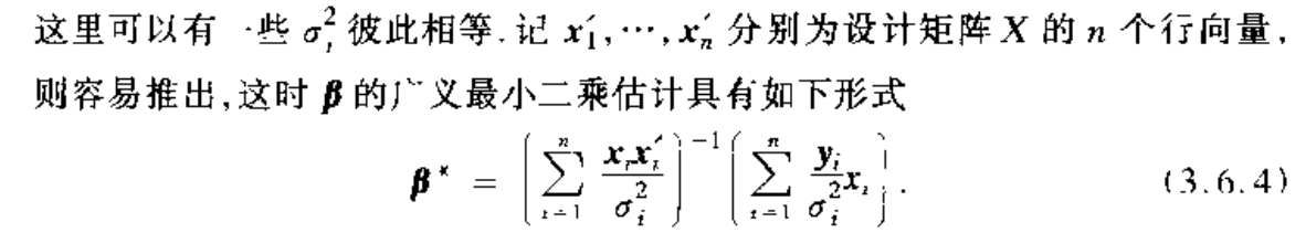
Example: a special form of generalized model
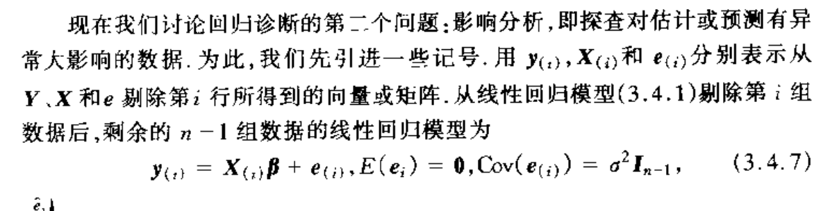
1.6. incomplete-data least square
Def: eliminate some row(s) of the data and see the difference of parameter vector .
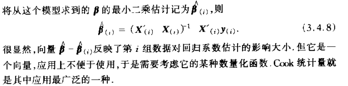
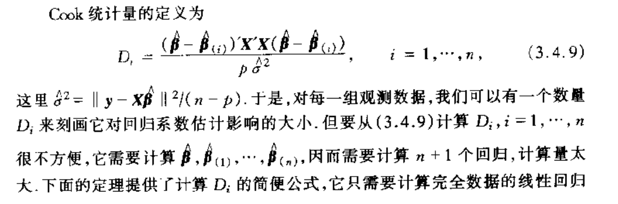
Def: cook stats,
Usage: a metric to rank the influence ( when we eliminate certain row of data)
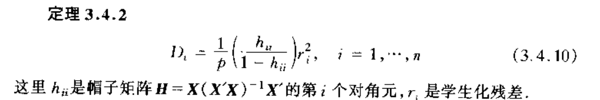
Theorem: => relationship between cook & student residual
Usage: we don't have to actually compute cook every now and then, using the theorem we can reduce the complexity by a large scale.
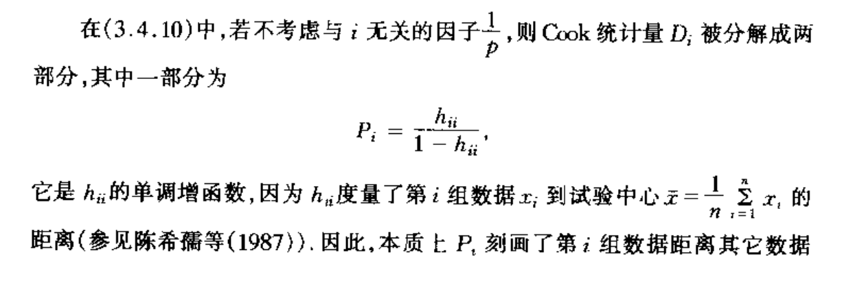
Note: intuition for cook.
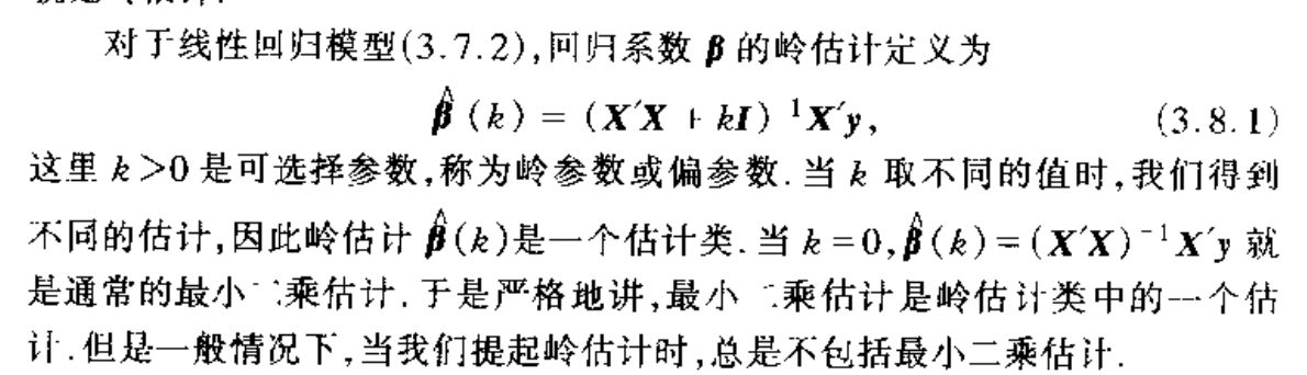
1.7. ridge least square
Def: model is the basic model
Algorithm: algorithm is different when k $$ 0
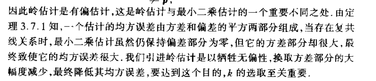
Note: why we need ridge regression
Def: regularized linear model
Algorithm: least square for reguoarized linear model


Qua: => Var

Qua: => relationship with basic model

Note:

1.7.1. MSE
Qua: => relationship of MSE with basic model
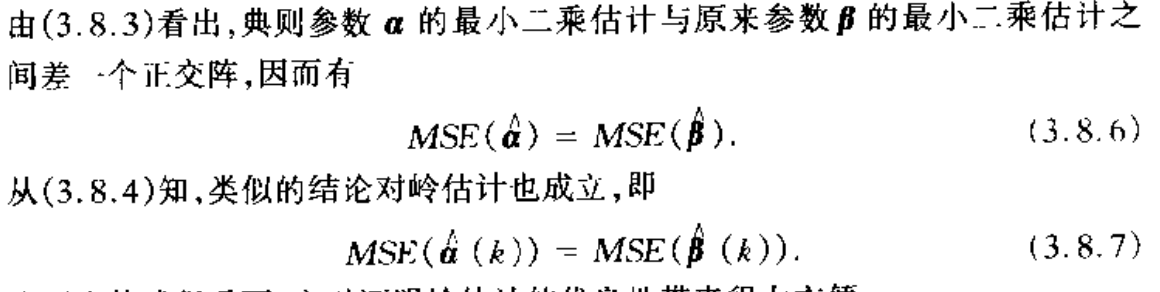
Qua: => MSE < basic model
Usage: this is why we choose ridge regression
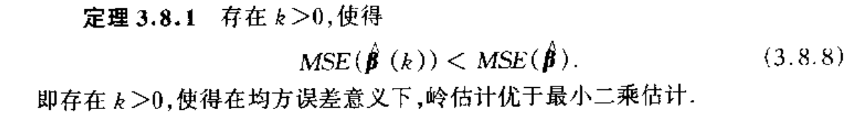
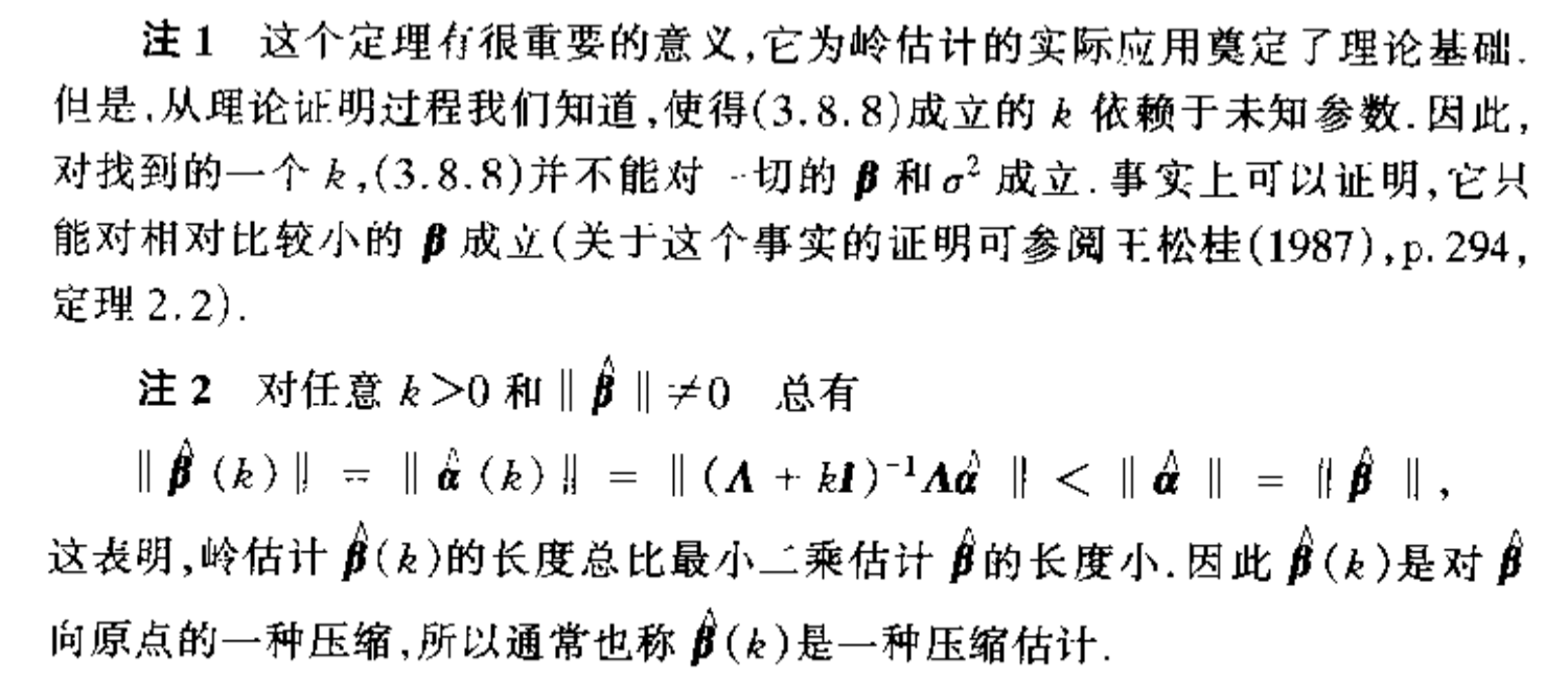
Note: this is a very important .
1.7.2. optimal K
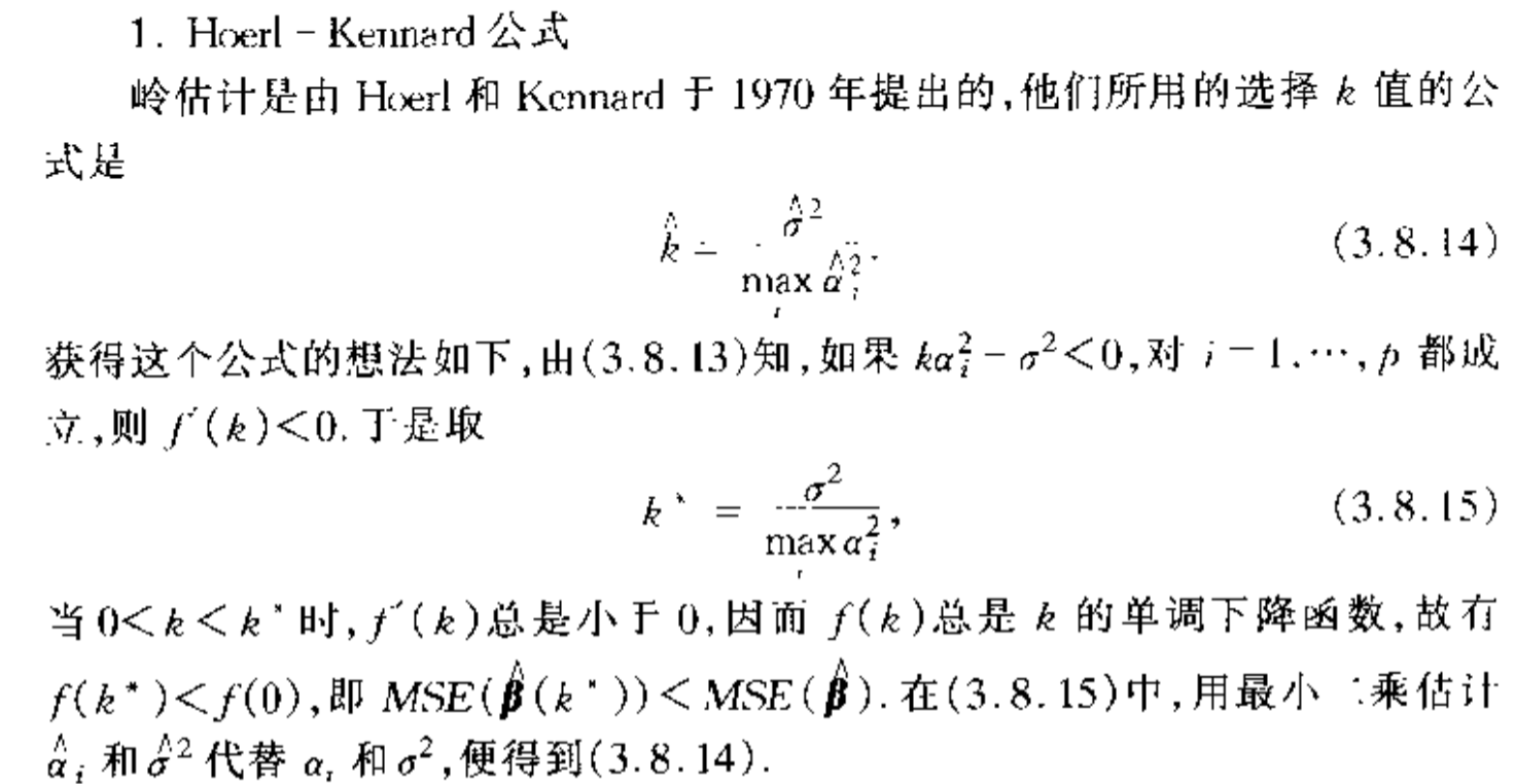
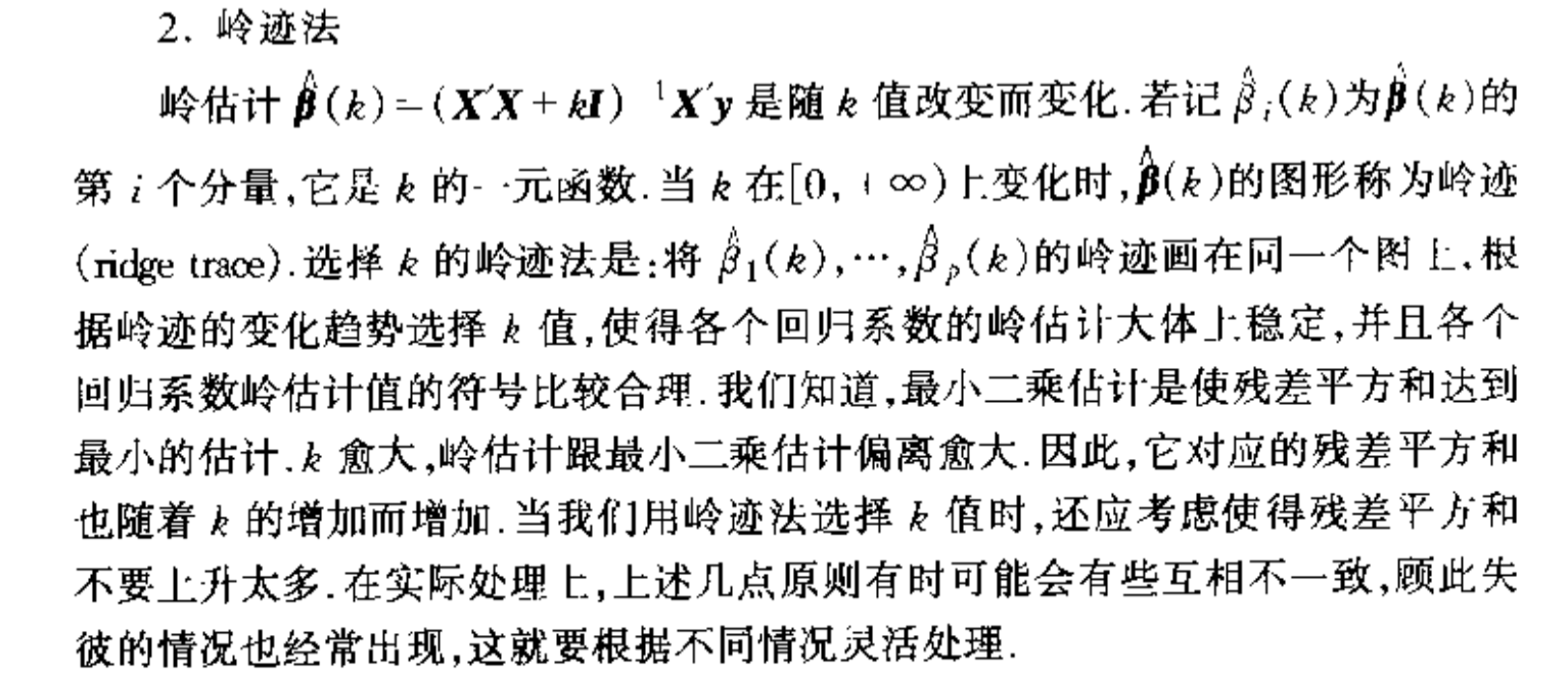
Algorithm: Hoerl-Kennard equation
Algorithm: ridge plot
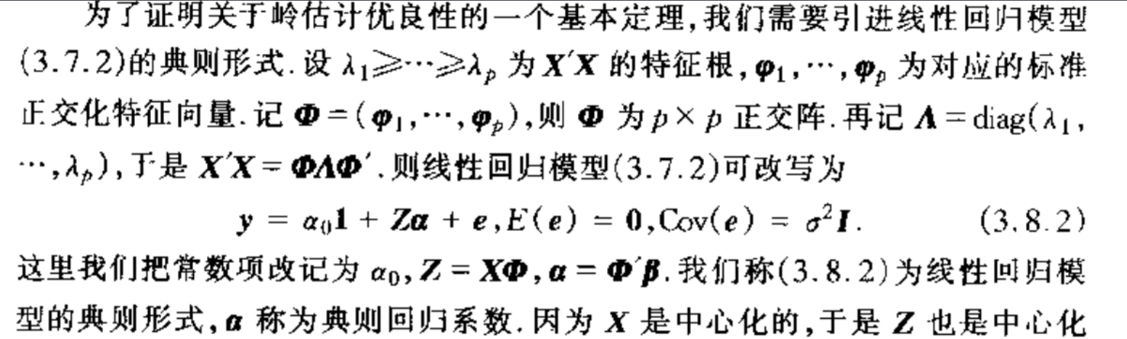
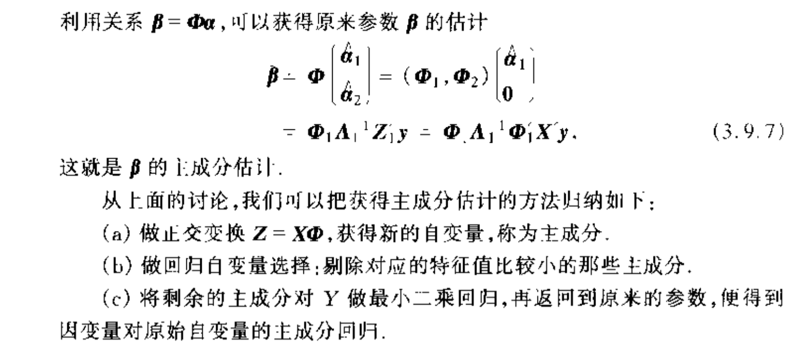
1.8. PCA regression
Def: PCA linear model
Usage: same as ridge regression, centralized!!

Def: first principle
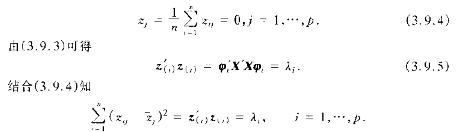
Qua: => relationship between Z and eigvalue
Intro: intuition for PAC regression: when eigvalue is small we eliminate it.

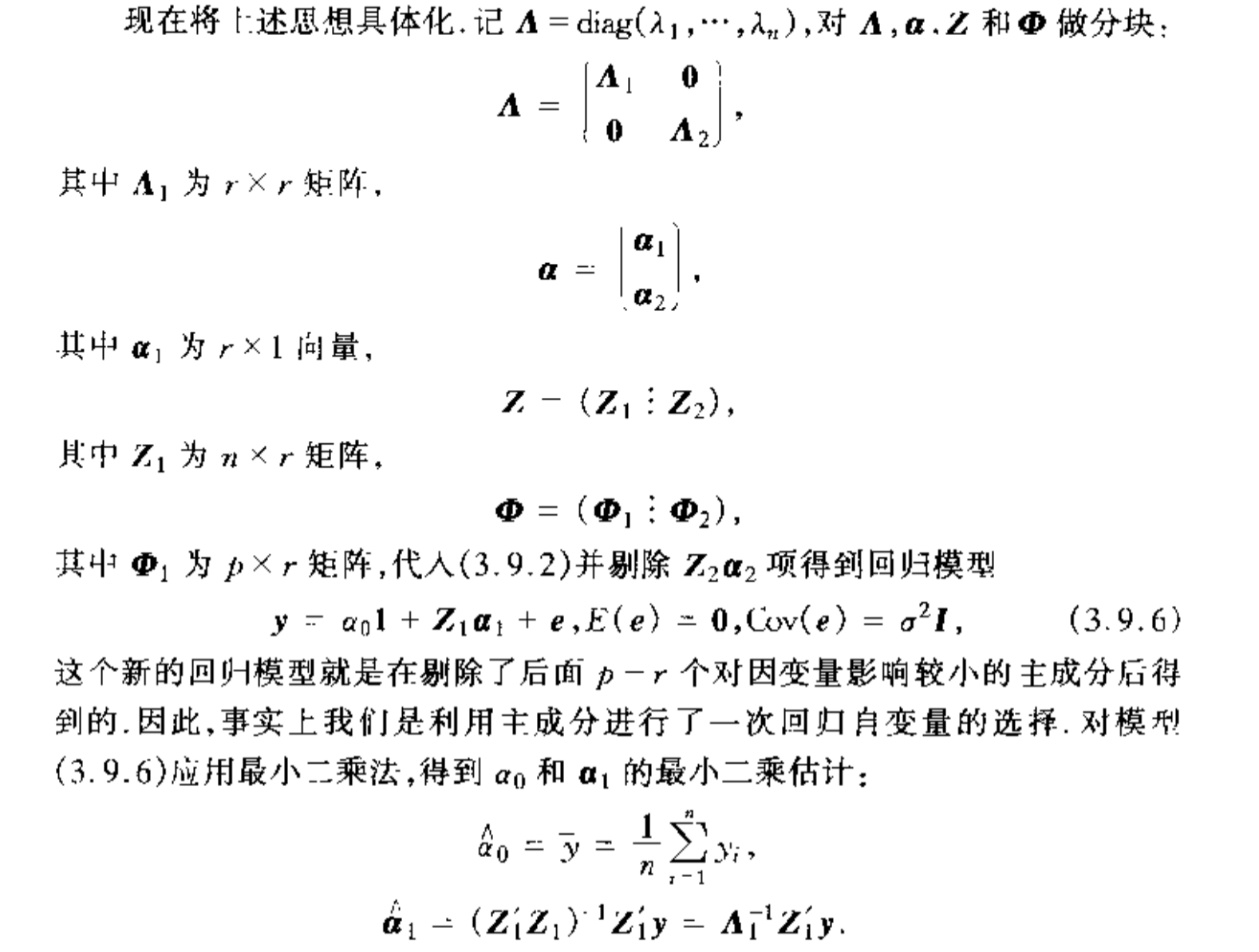
Algorithm: PAC regression: similar to regularized model except that we eliminate some part of Z.
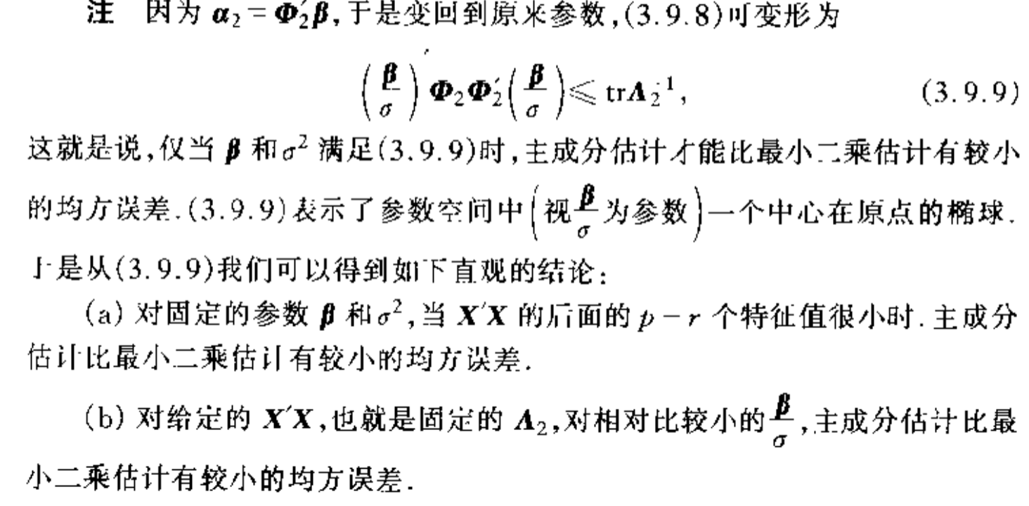
1.8.1. MSE
Theorem: we can also decrease MSE by PCA regression
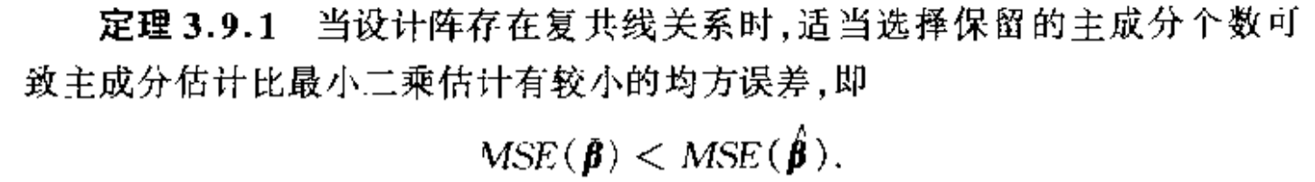
Note: there's condition to this theorem
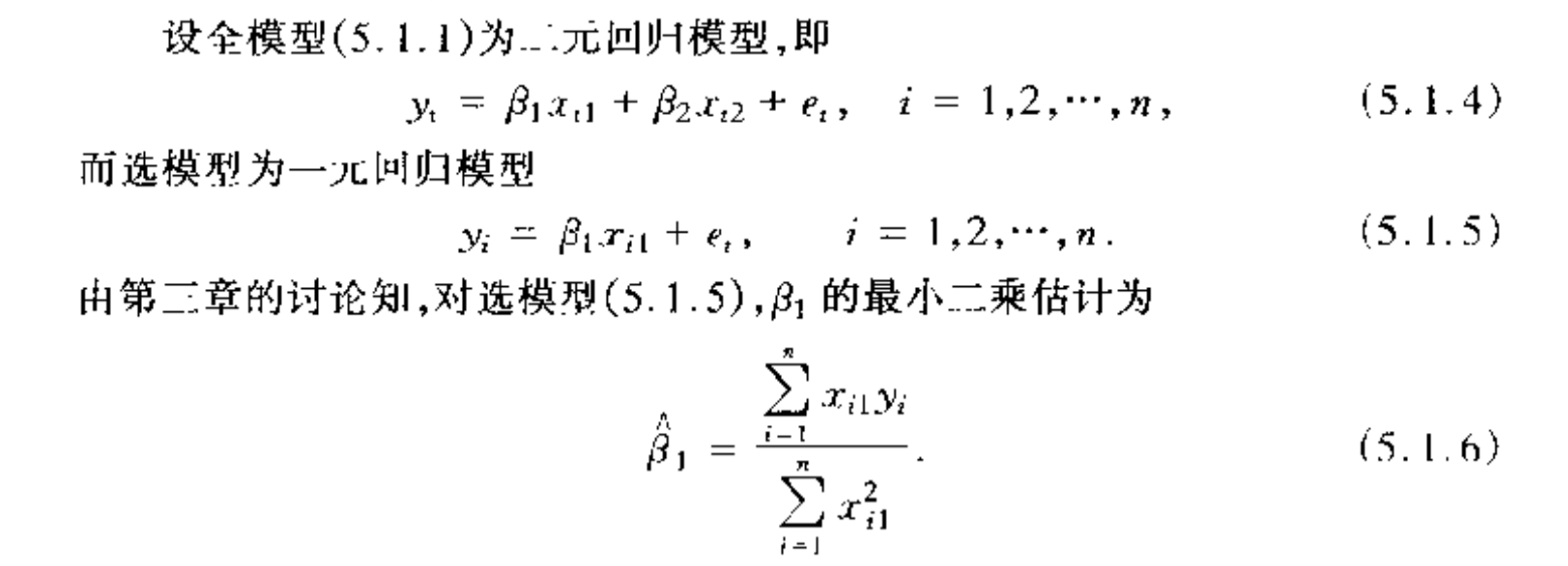
1.9. imcomplete-feature least square
Def: model
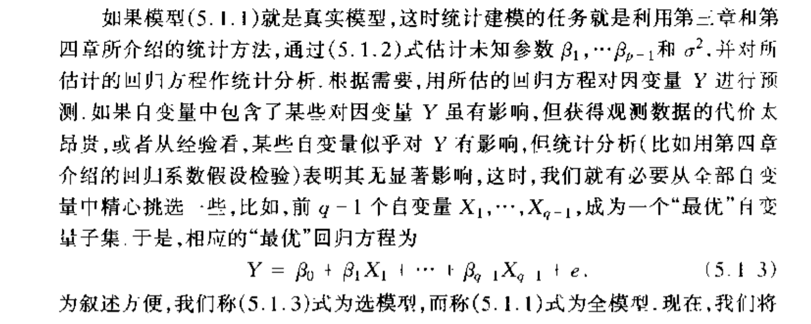
Algorithm: least square (notice the difference here between 1.9, in 1.10 we assume we don't know which is the correct model, in 1.9 we assume we know which is the correct model.)
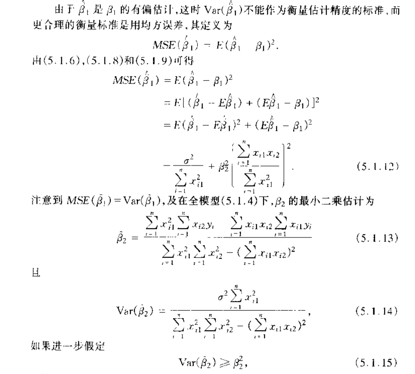
1.9.1. expectation & var
Theorem: => biased E and Var

Proof: P103
1.9.2. MSE
Theorem: => MSE smaller
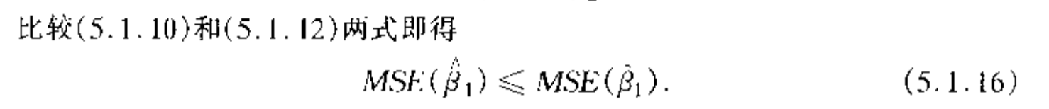
Proof:
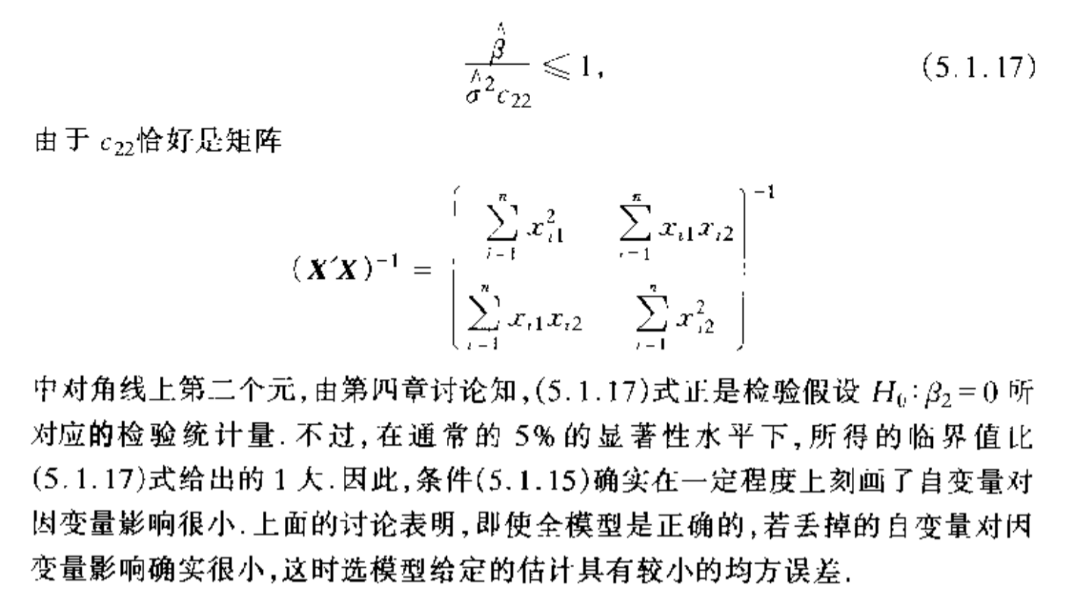
Note: the condition(5.1.14) is not always correct:

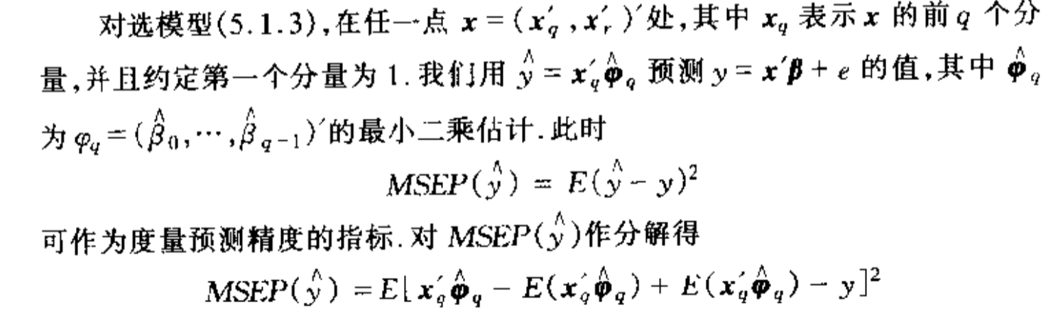
1.9.3. prediction problem
Def: prediction problem
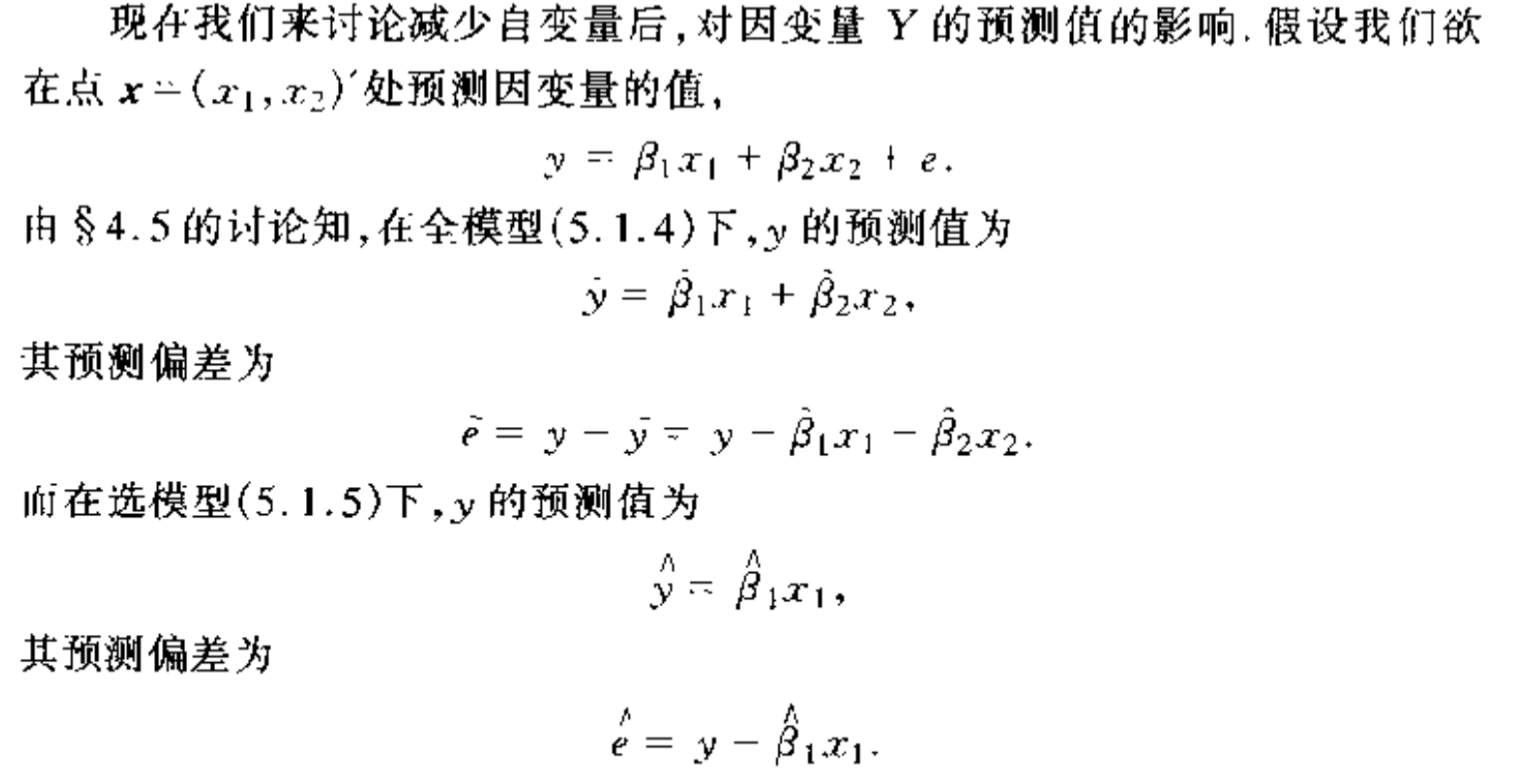
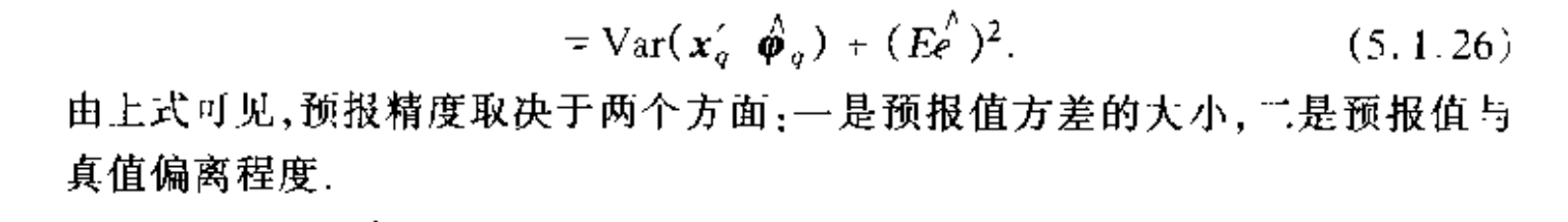
Qua: => using MSEP we yield this

Proof: see P108
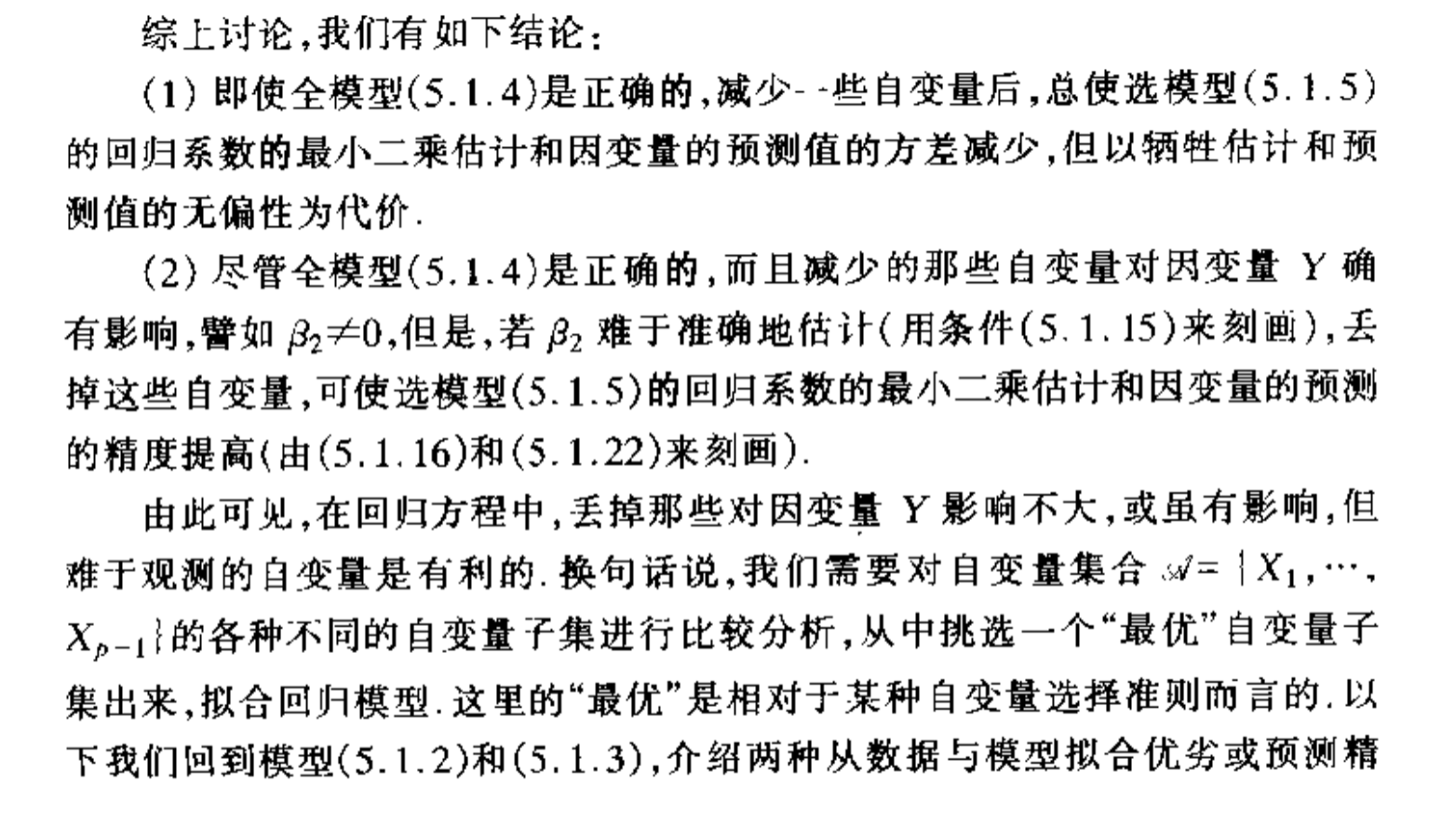
1.9.4. conclusion
Note: conclusion for above 3 sections
1.10. non-linear regression
2. regression analysis
2.1. cook distance
Def: introduced in 1.7
Usage: strong influence/ outliers
2.2. VIF/ CI
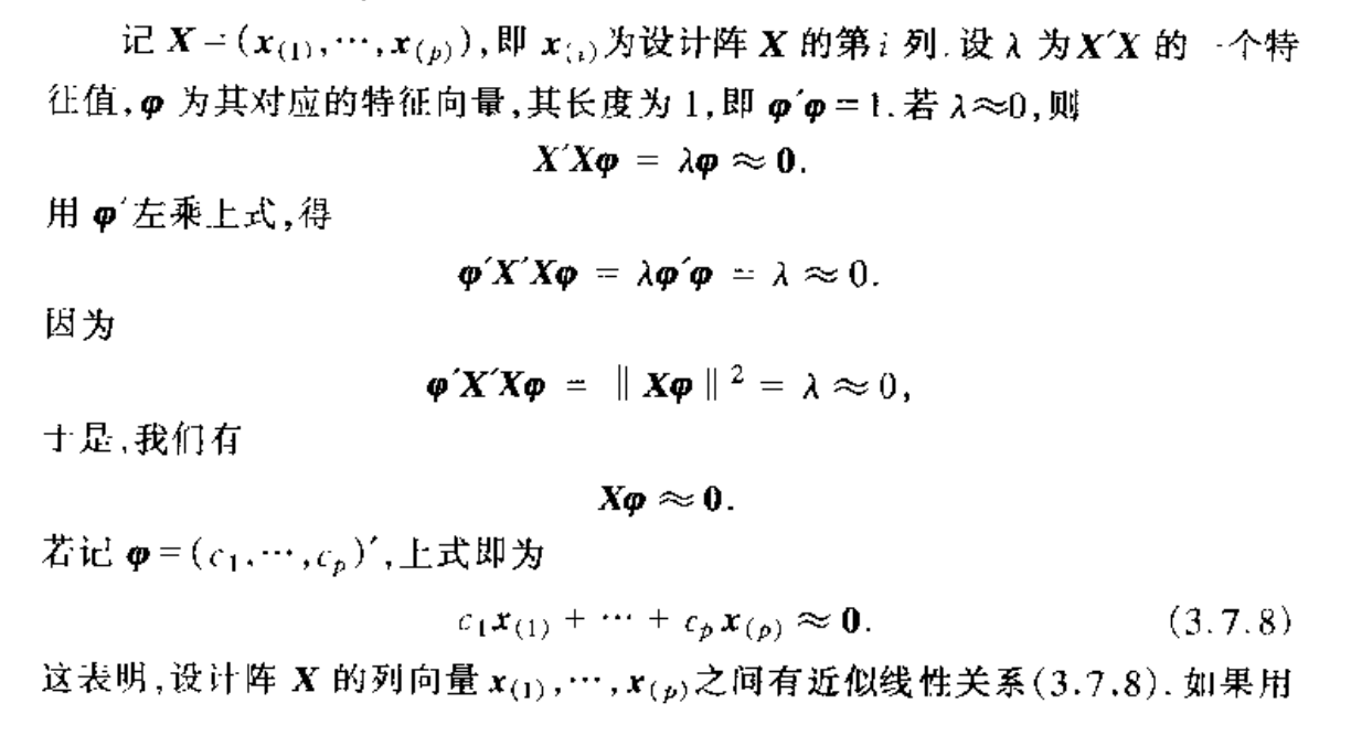
Intro: in 1.3.2 we know that MSE is corresponding with eigvalue, now we show that what does eigvalue mean in linear model
Def: multicollinearity

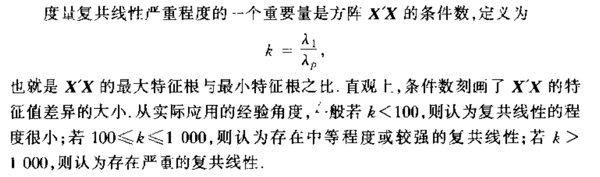
Def: CI
Usage: tool to show how severe is multilinear
Def: VIF
Usage: same \[ \frac{1}{1-R_j^2} \]
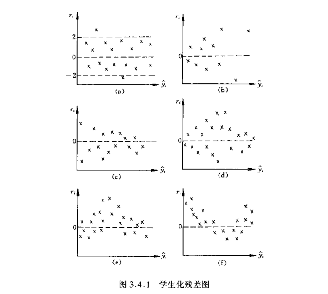
2.3. student resitual map
Def: student residual
Usage: a standardized form of residual vector
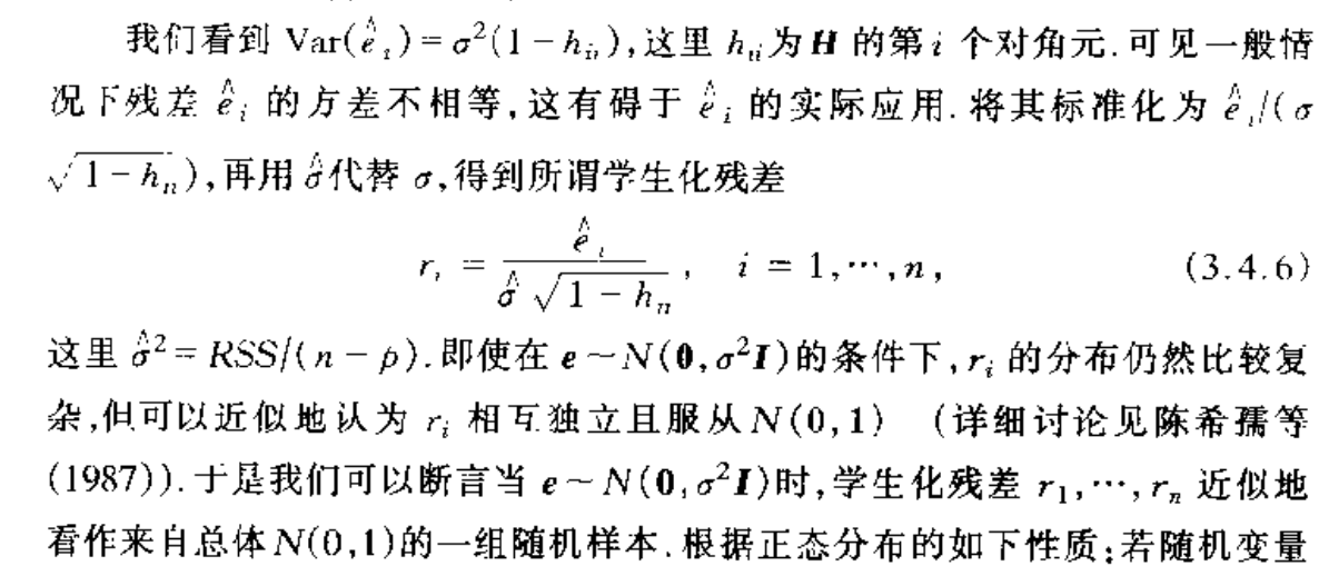
Algorithm: student residual plot
Usage: all hypothesis

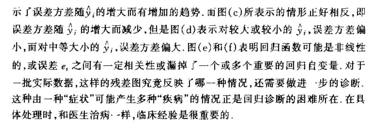
Note: 6 types of residual map
2.4. Box-cox transformation
Def: Box-cox transformation
Usage: all conditions
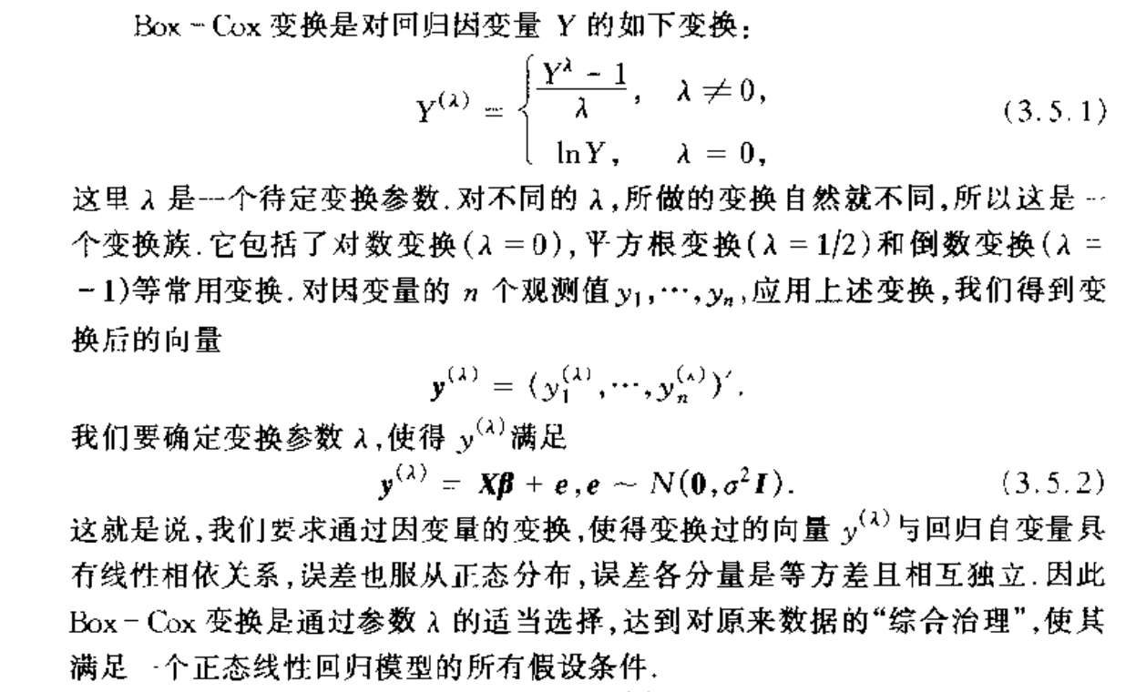
Algorithm: mle for optimizing the optimal \(\lambda\)
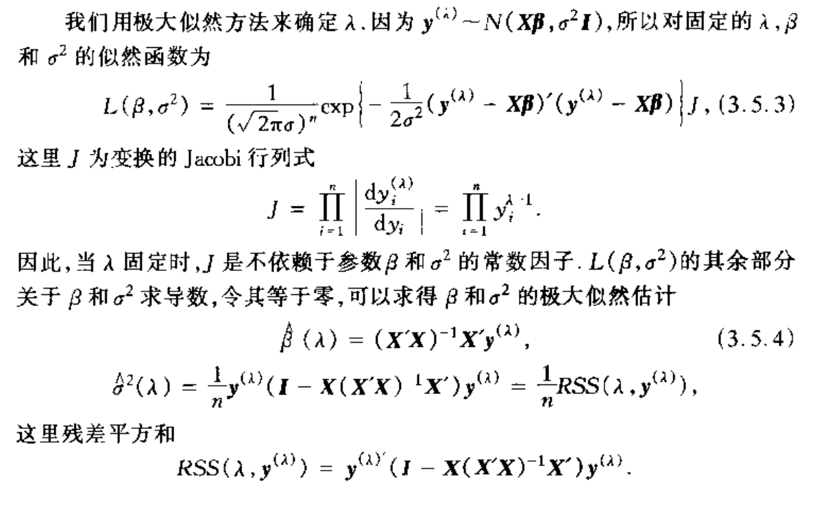
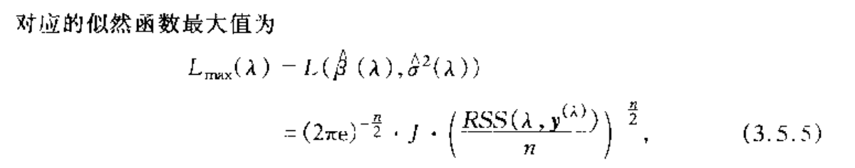
Note: basic tranformation to log maximization problem
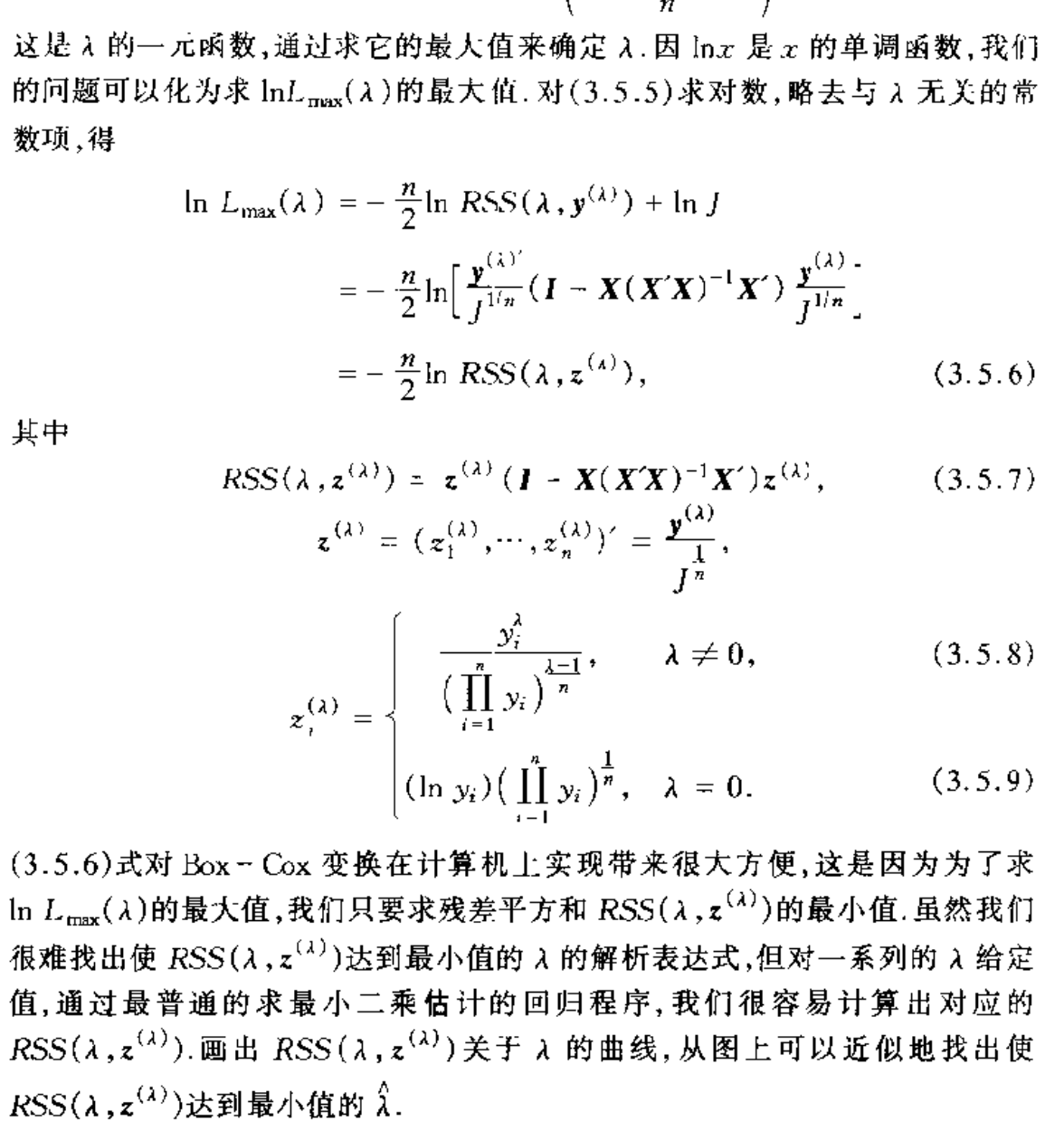
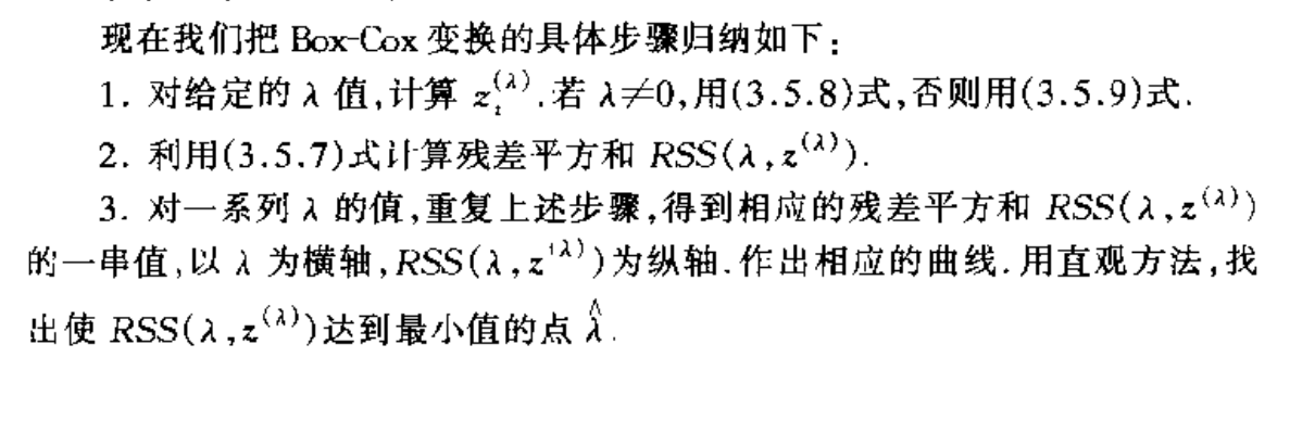
Note: oveall brief algorithm

3. regression hypothesis test
3.1. linear test
Def: basic linear test

Note: basic idea to this test
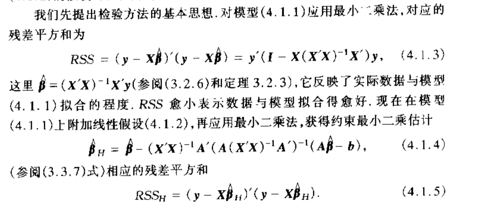
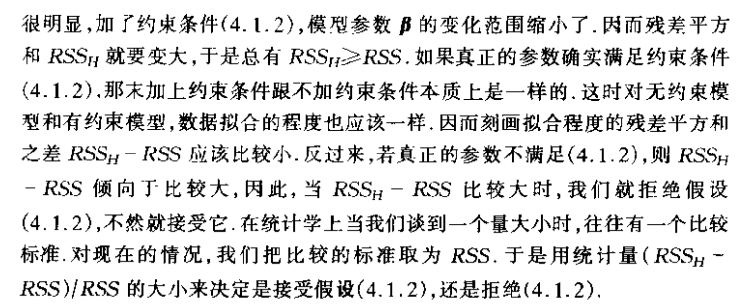
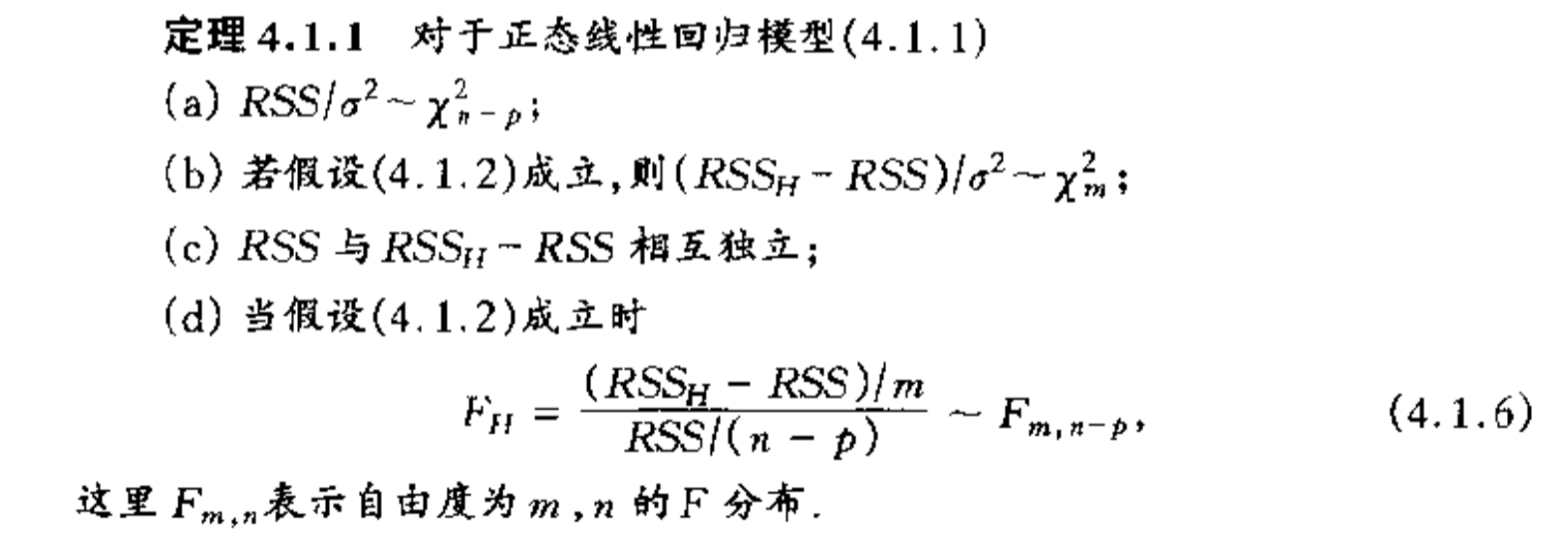
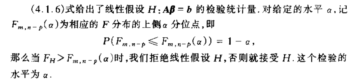
Algorithm: the test
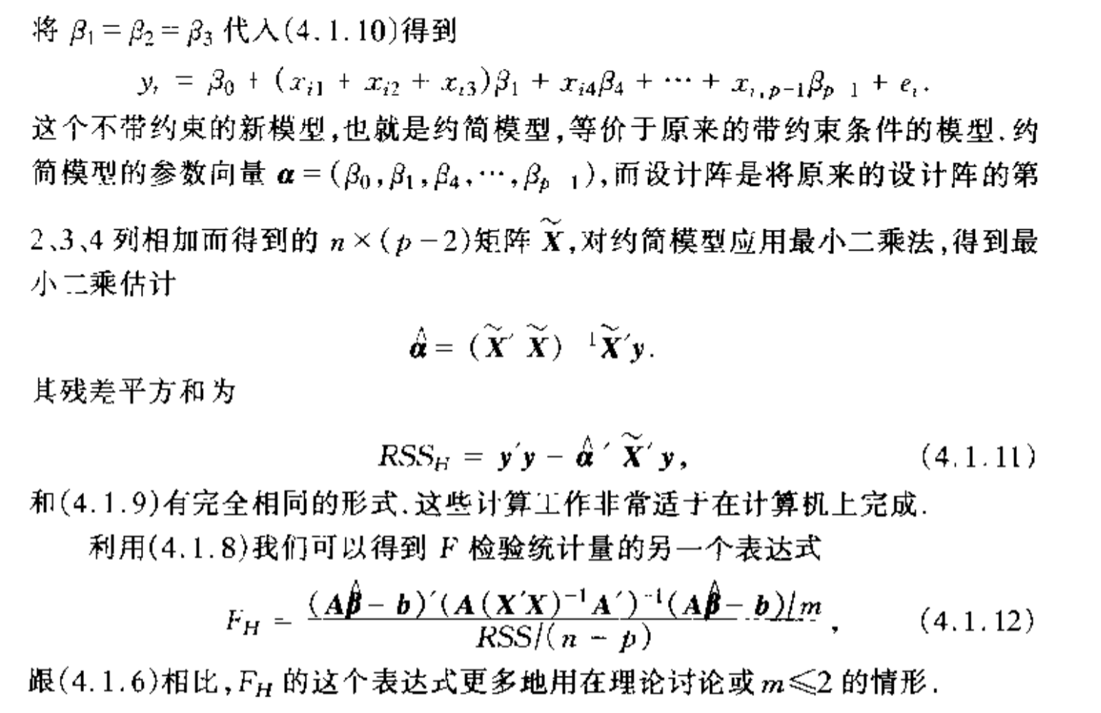
Note: we can simplify the test since \(RSS_h\) are hard to compute : by using a 约减 model (putting AX=b into the model and make it unconstraint)

3.2. model test
Def: model test
Usage: which is a special test of section 3.1, but we'll make it simpler
Note:
Algorithm: the same thing as 3.1
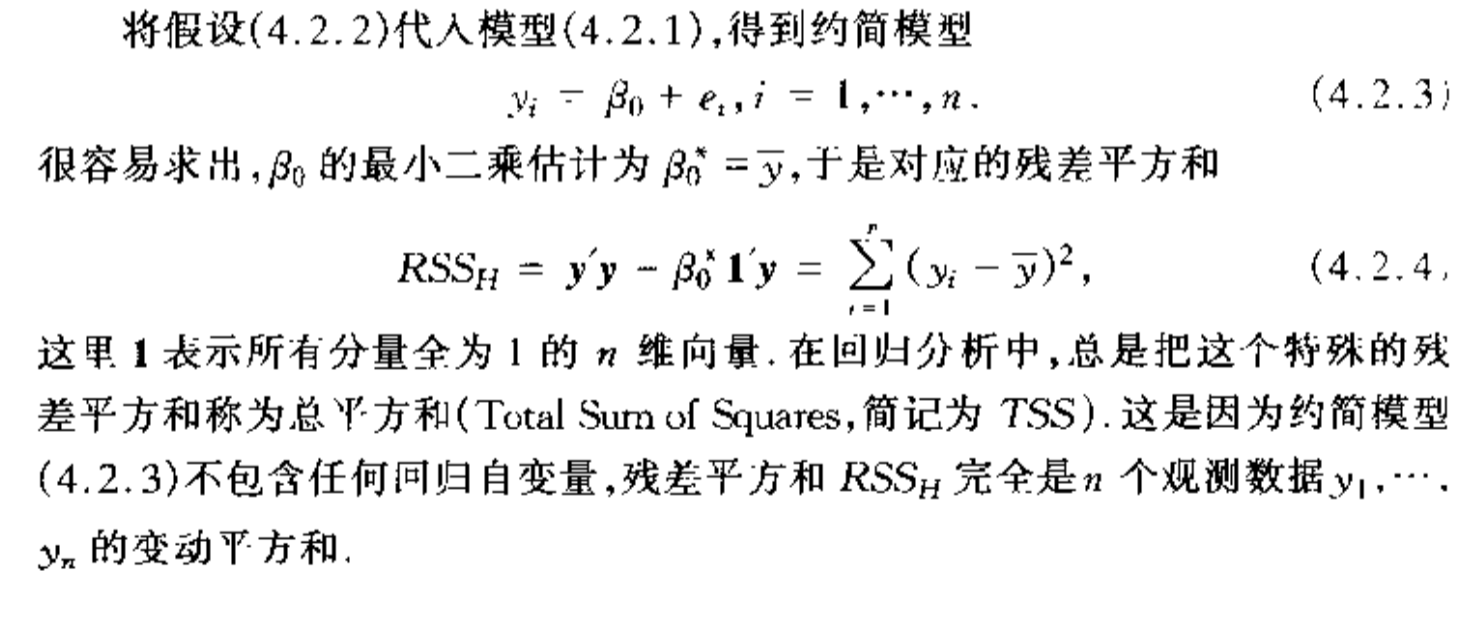
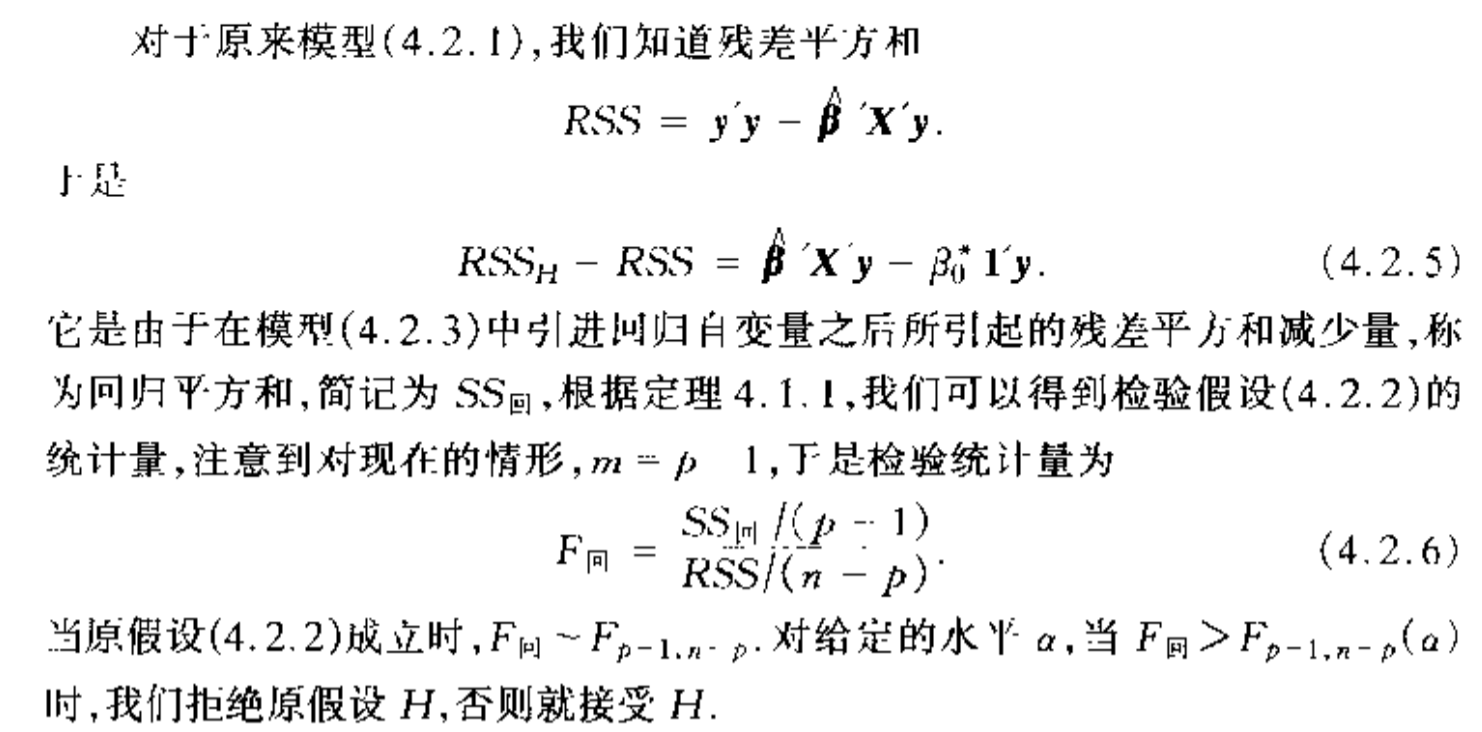
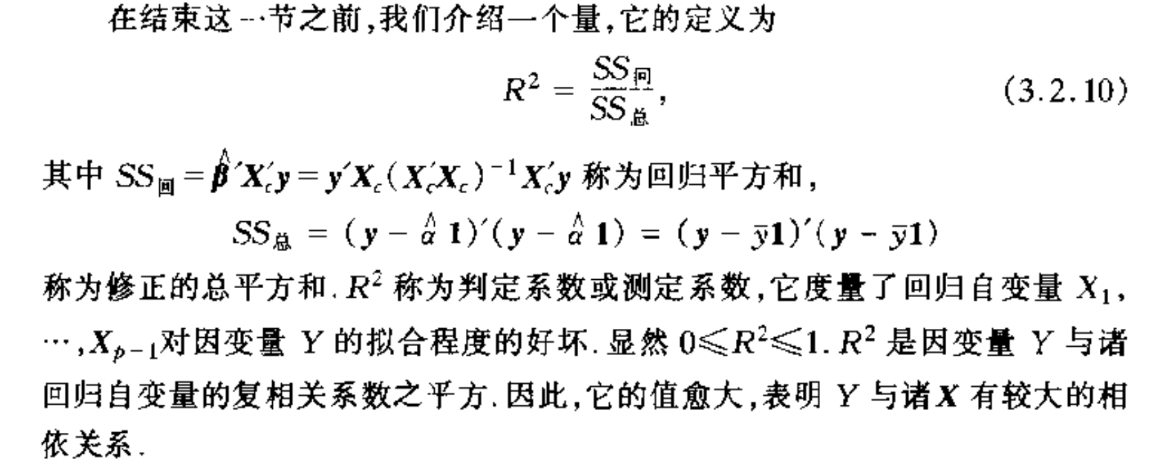
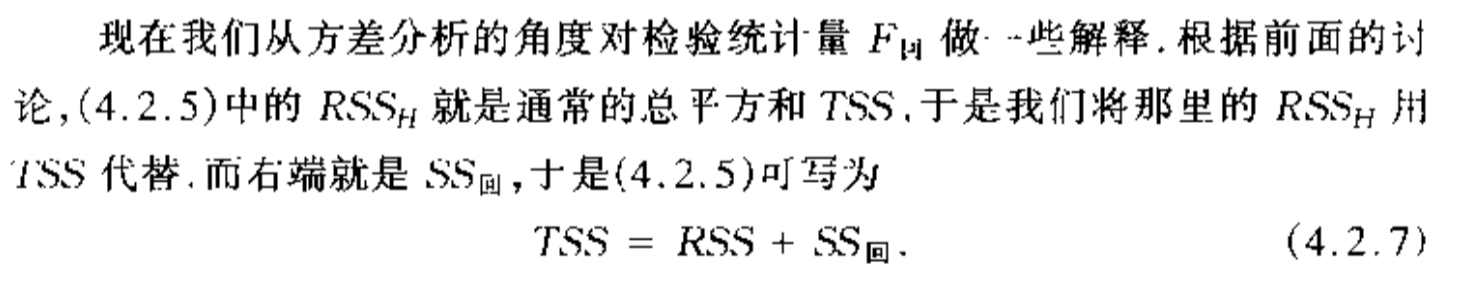
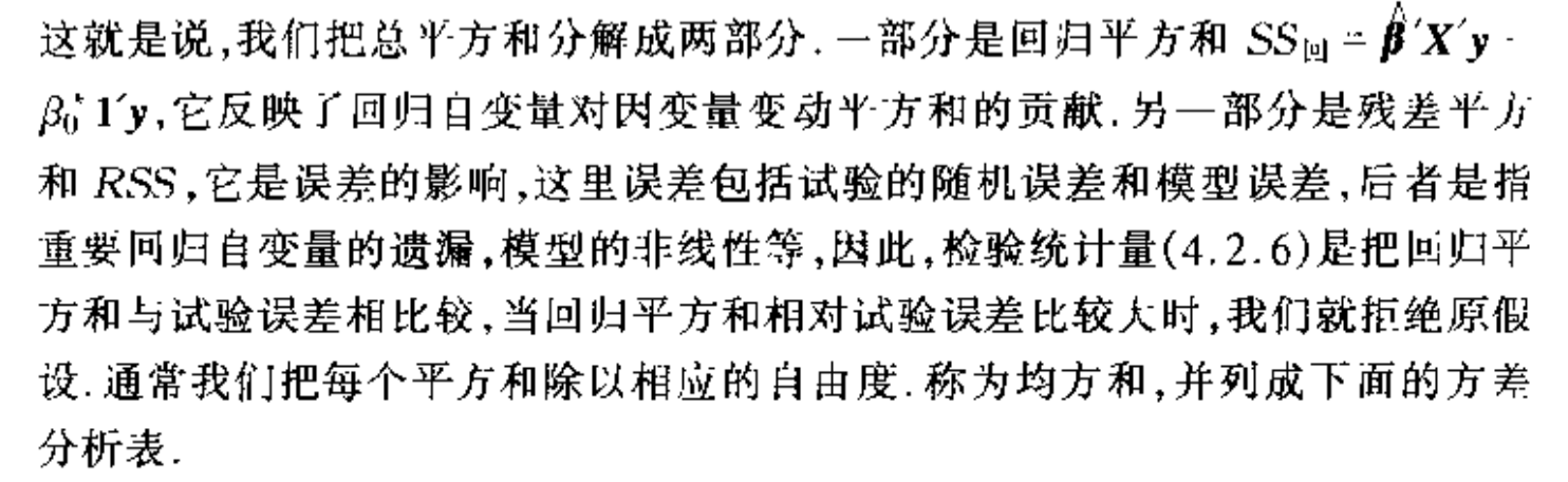
Note: the famout TSS = RSS +ESS equation
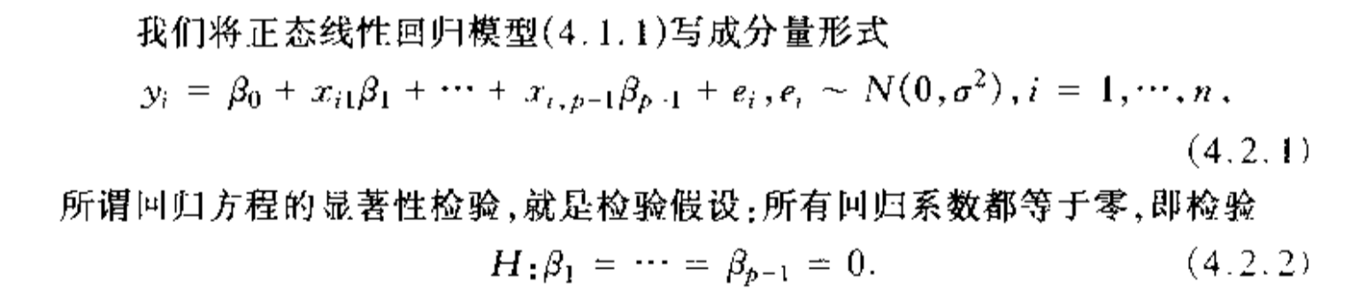
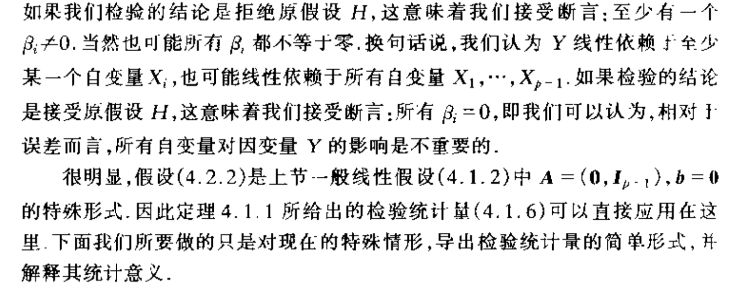
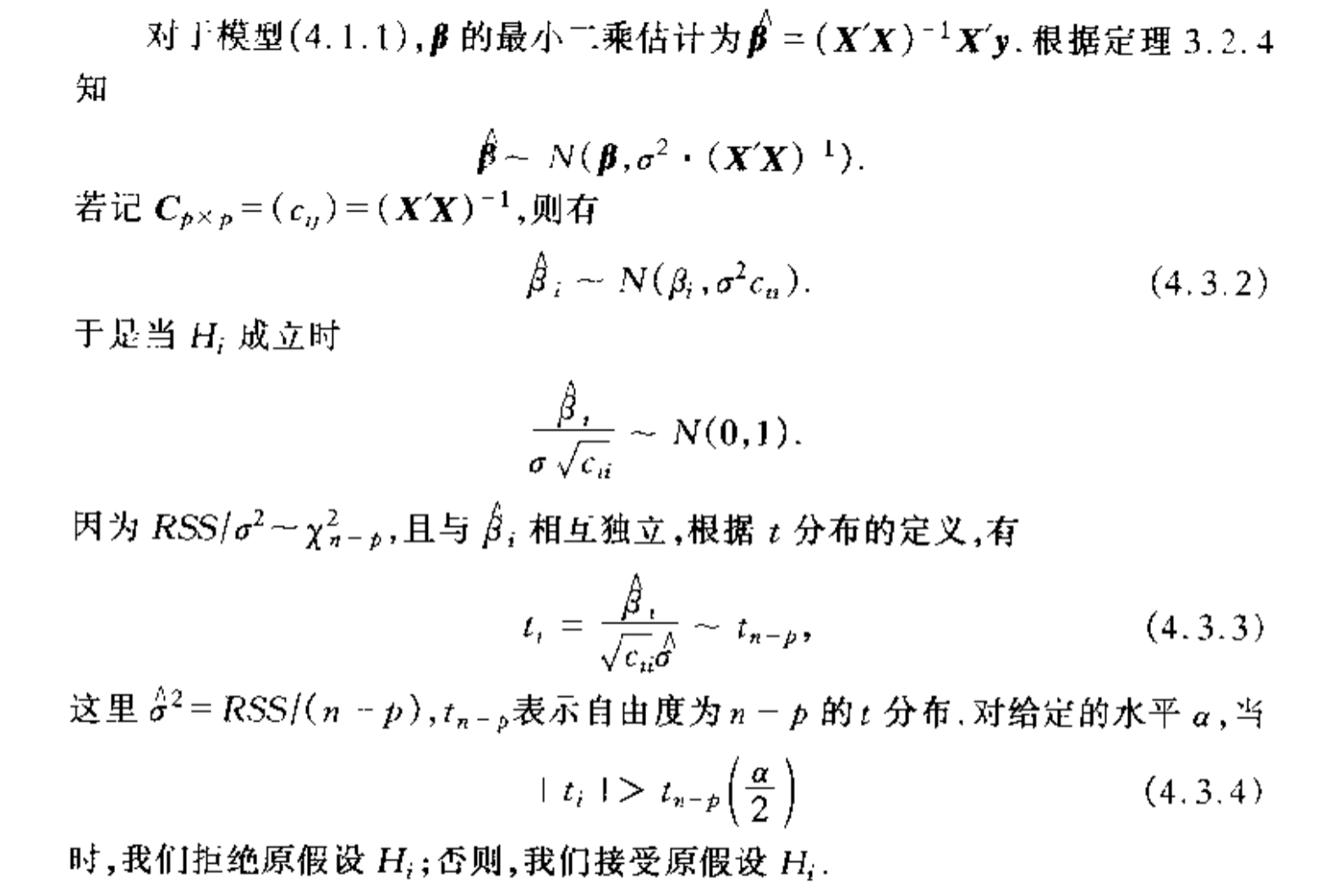
3.3. saliency test
Def: saliency test ( a special form of 3.1 but we'll give a simpler way)
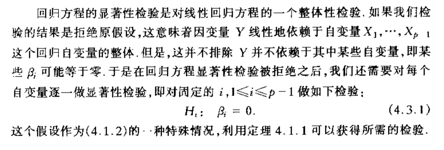
Algorithm: saliency test
Note:

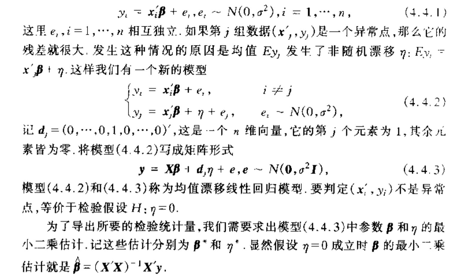
3.4. outlier test
Def: outlier test
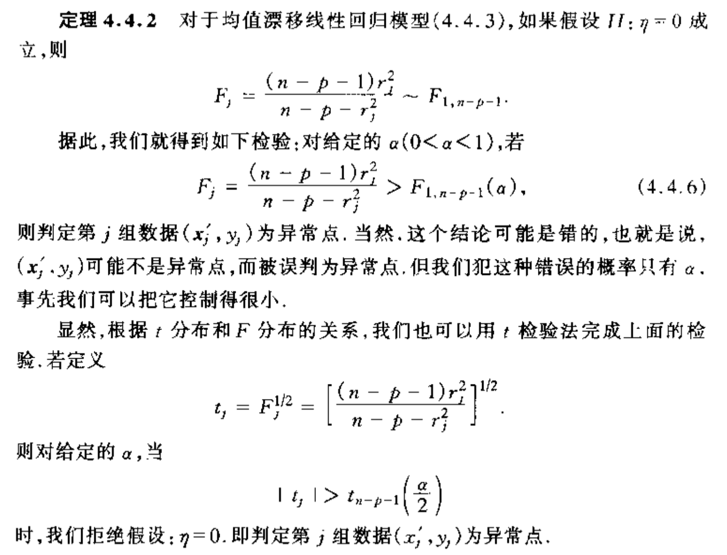
Theorem:
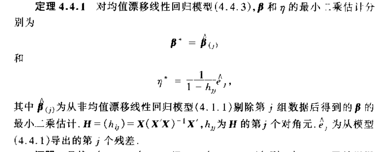
Note:

Algorithm:
Proof:


3.5. the prediction problem
3.5.1. point estimation
Def:

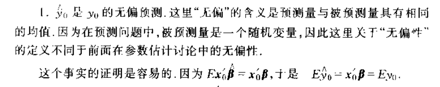
Qua: => unbiased
Qua: => markov

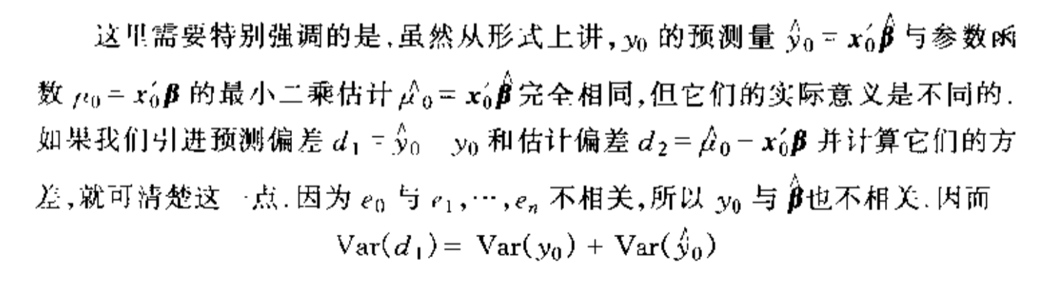
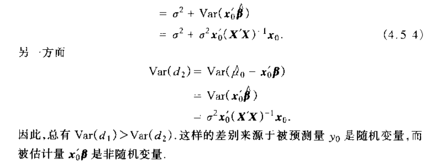
Qua: difference between
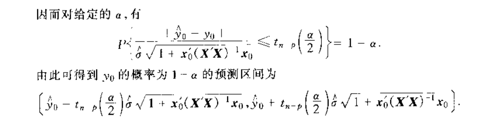
3.5.2. interval estimation
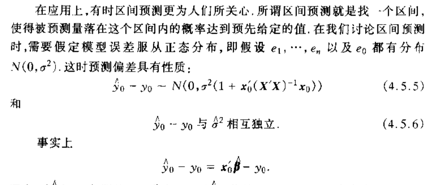
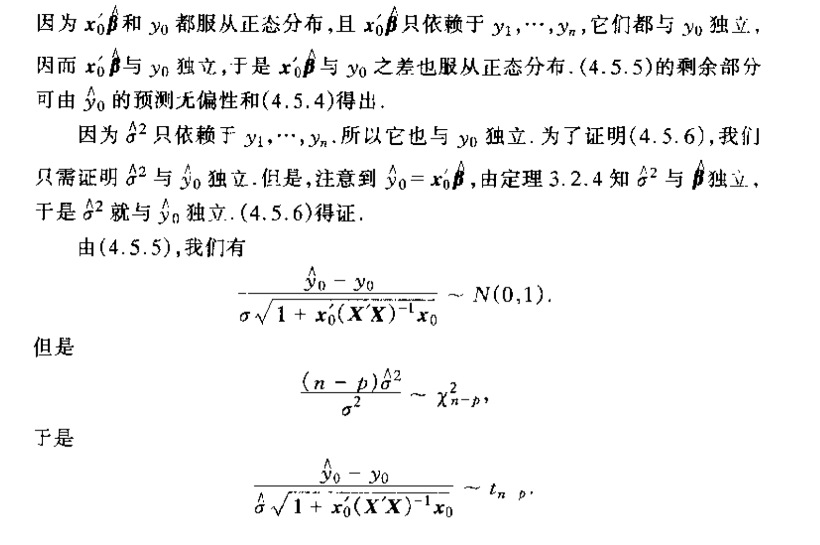
Def:
4. regression feature selection
## metrics for selection
Def: Rssq ( the \(q_{th}\) time of selection)
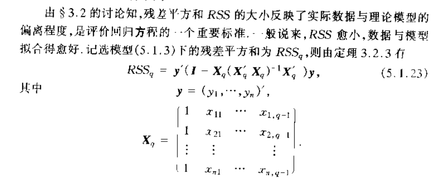
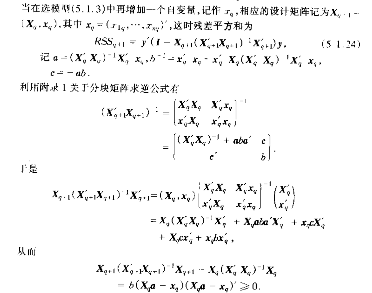
Theorem: => Rss q > Rss q+1
Usage: which means the more feature we choose the more accuracy we'll get.

Proof:
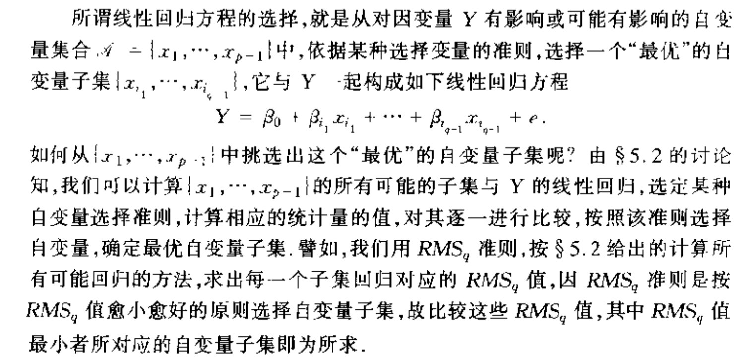
Def: \(Rms_q\)
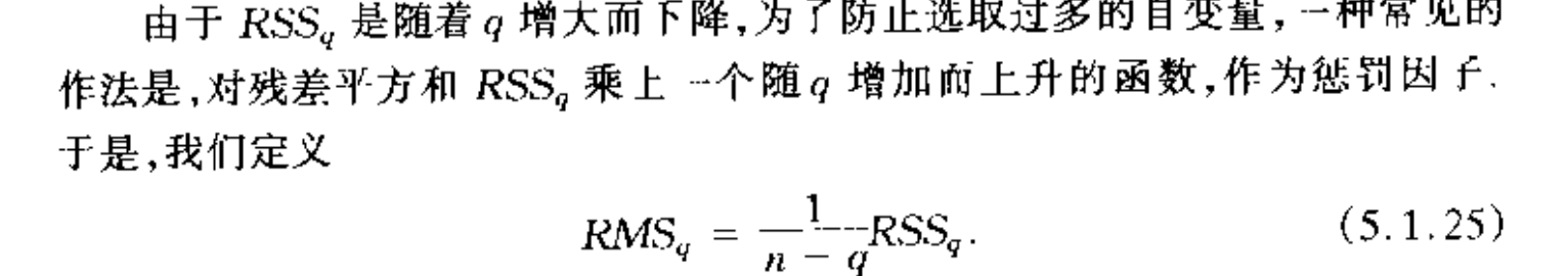
Note: the smaller RMSq, the better is the model

Def: MSEP
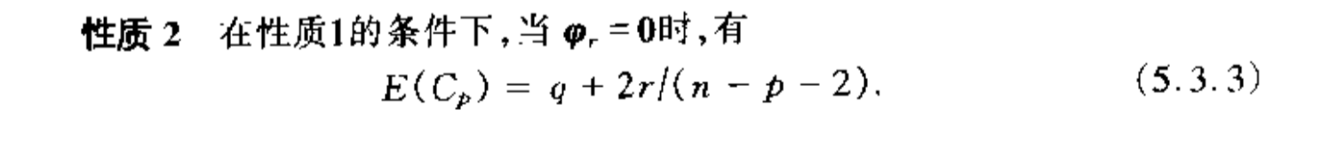
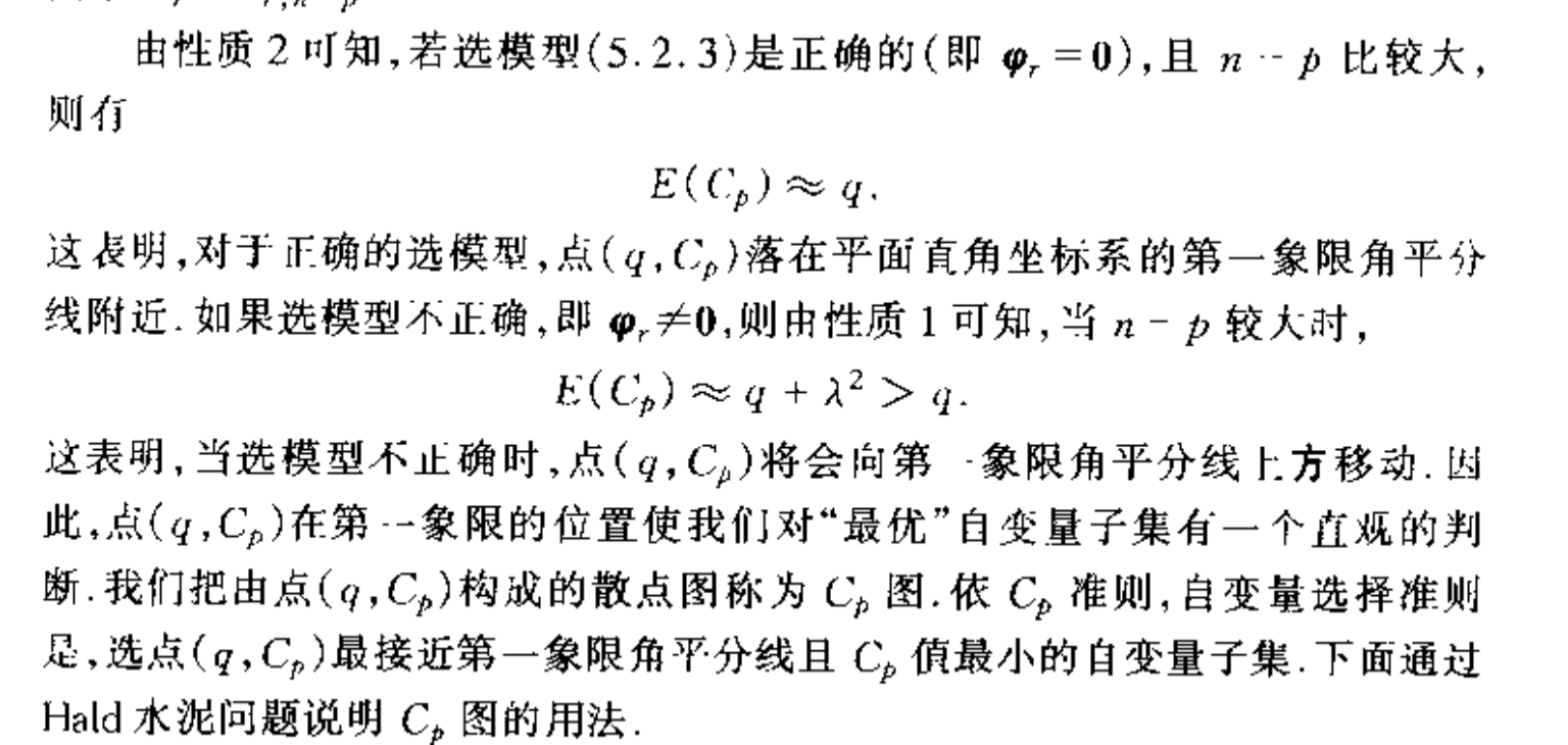
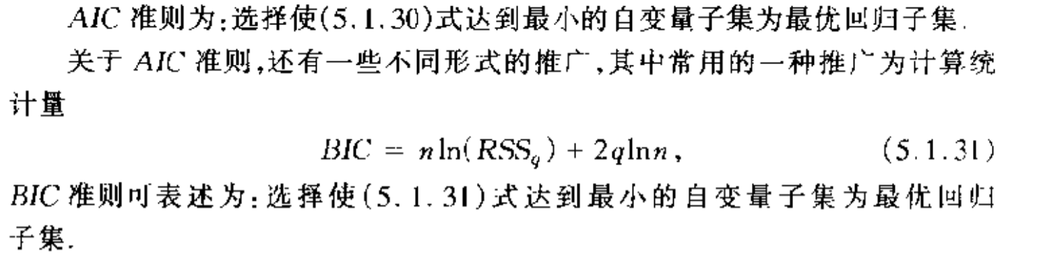
Def: CP
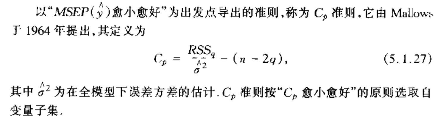
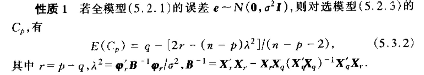
Qua: => no proof
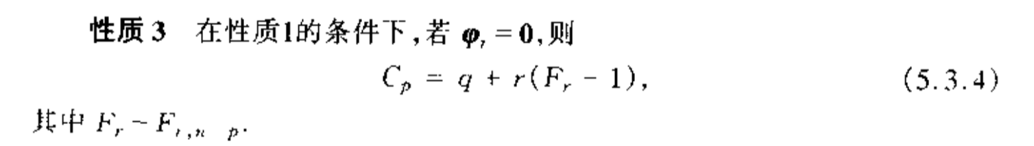
Note: we can plot to see if selection is optimal
Def: AIC( an application of MLE)
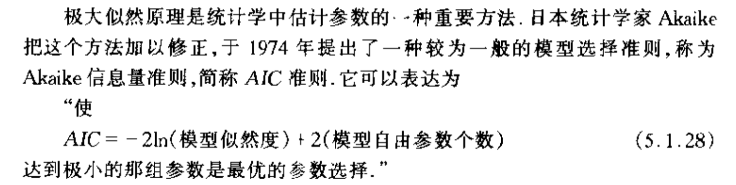
Note: specifically in linear model

Proof:
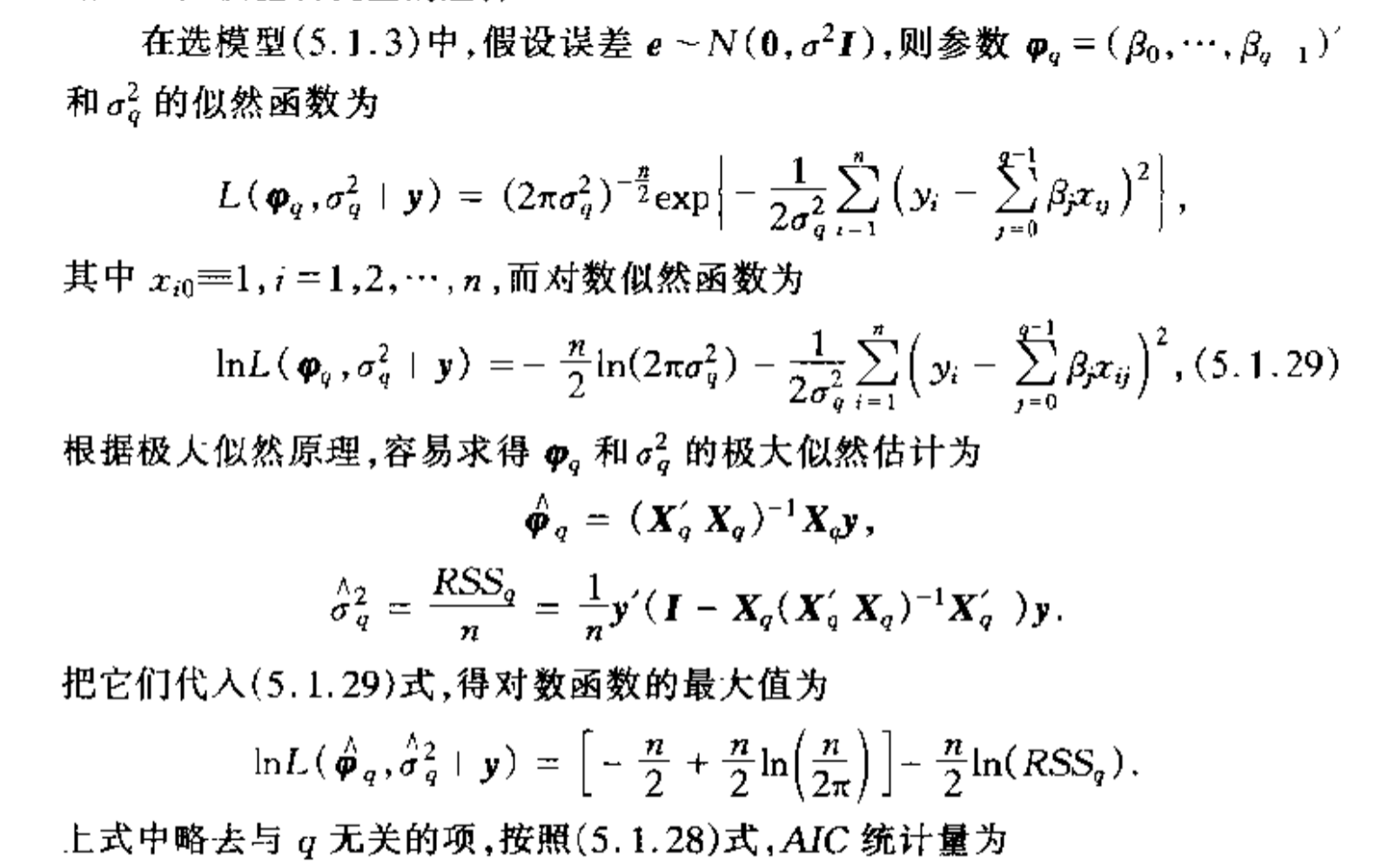
Note: the smaller the better
## optimal selection
Def: the best features
Algorithm: Cp plot
4.1. step-wise selection
- Algorithm: P149, basically do F test every step.