CS problems
1. general optimization problems
1.1. subset sum
Def: decistion form

Note: opt form, is a subproblem of backpack
maximum

minimum

k-subsum

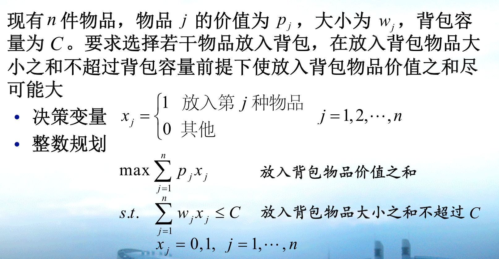
1.2. backpack problem
Def: 0-1 backpack problem
1.2.1. dp1
Algo: dynamic programming
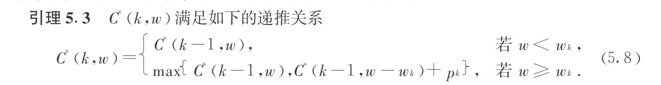
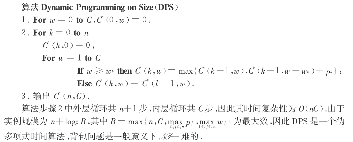
Qua: O(nC), pseudo-poly algorithm( if max number C is bounded by O(2^n), then the DP is polynomial, this is the definition of pseudo-poly)
the input is n+logL, L = max(max pj, max wj, C)
1.2.2. dp2
Algo: dynamic programming 2
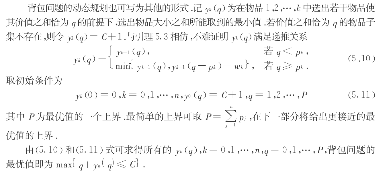
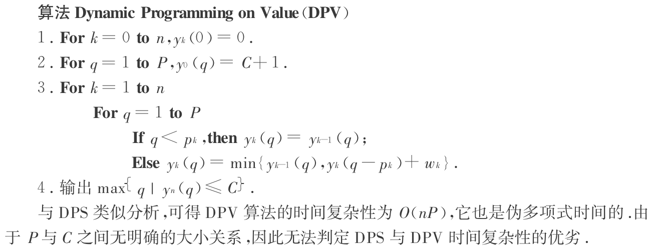
- Qua: O(nP), same as above
1.2.3. branch & bound
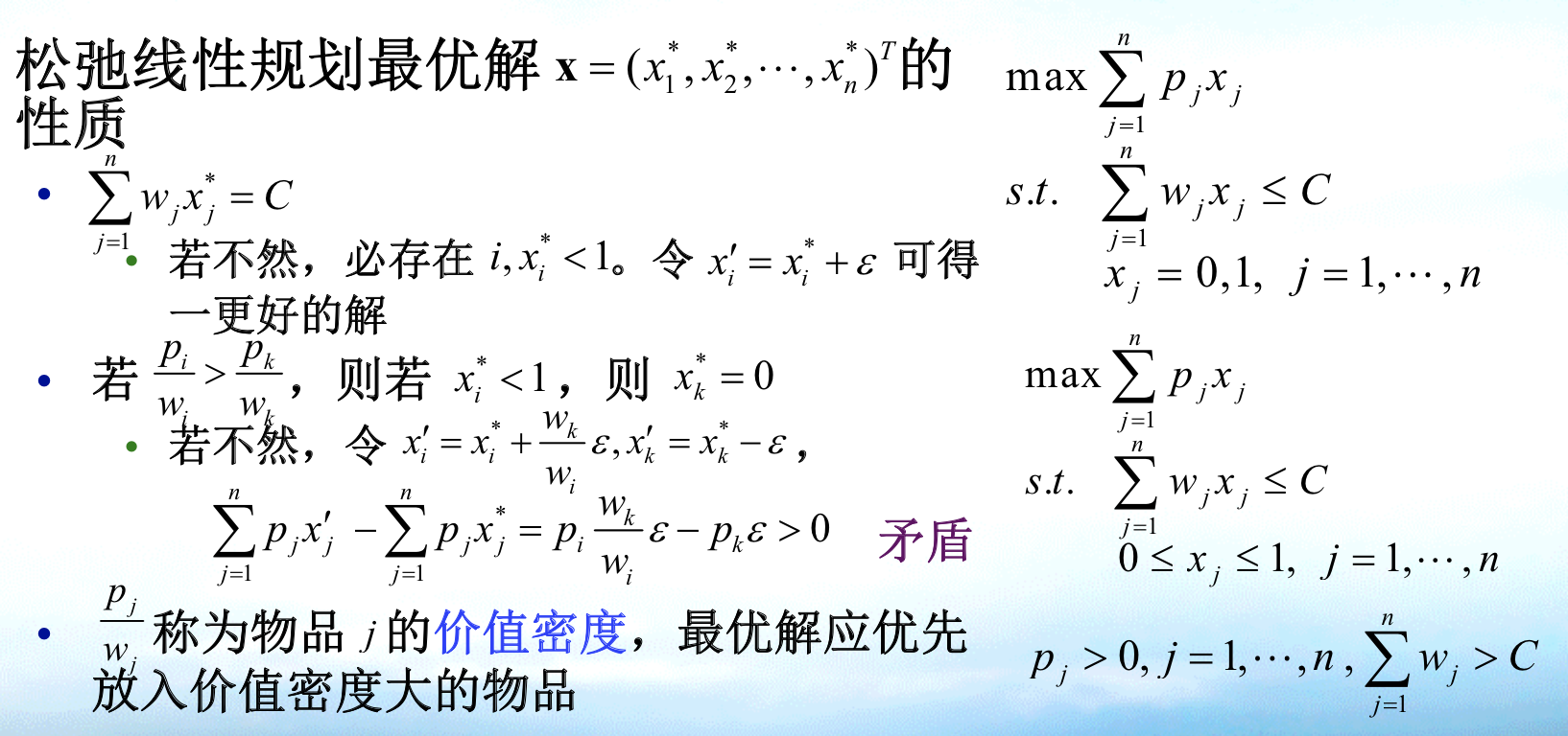
Algorithm: relaxation linear programming ( branch & bound method )
properties for relaxation problem
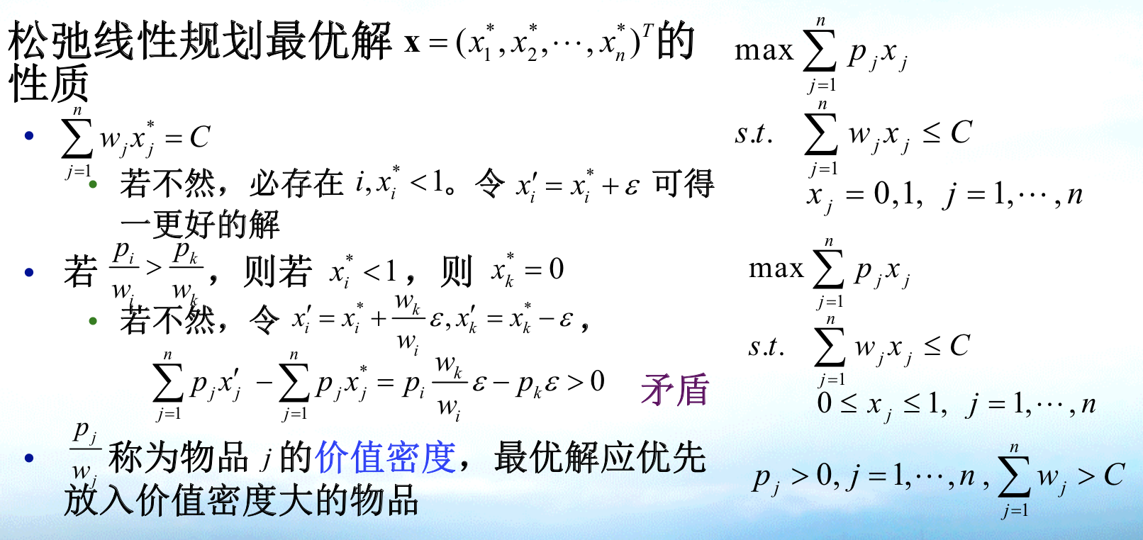
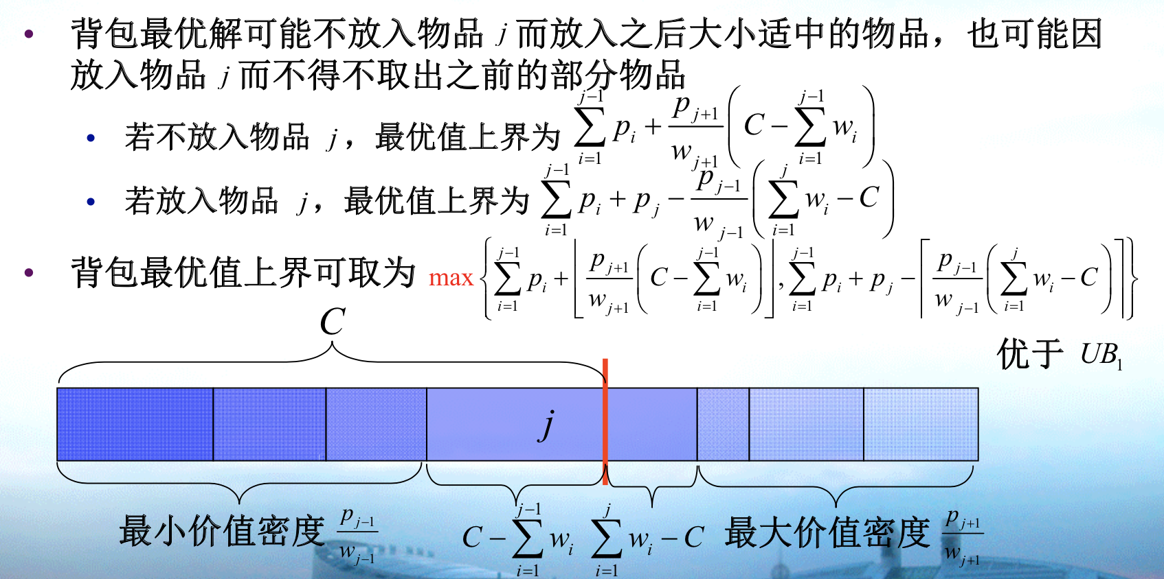
UB1: we use relation problem tp compute upper bound for non-relaxation, a fixed one, not optimal since we want it to be small.
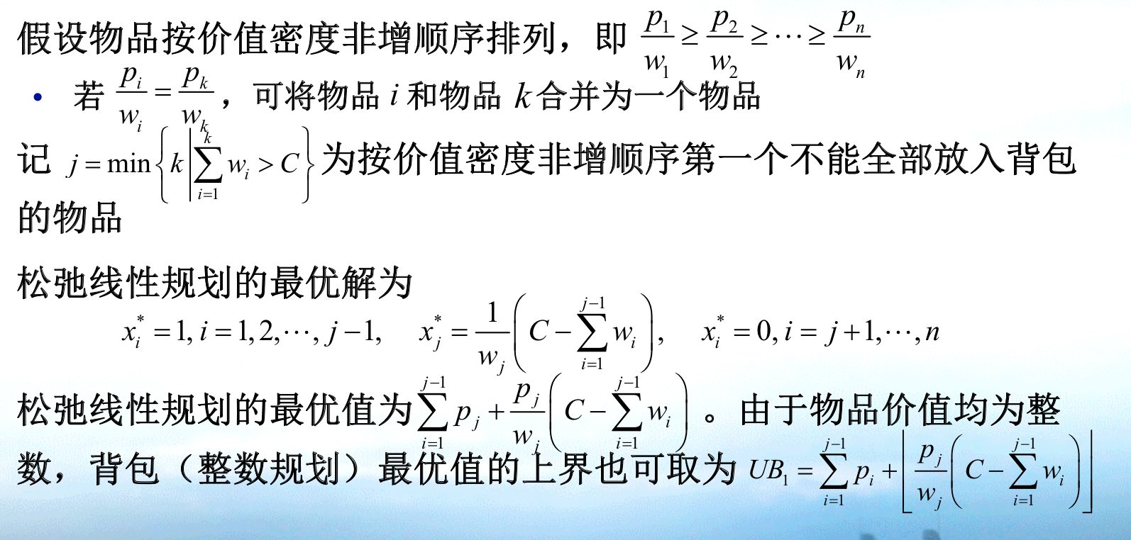
UB2: we optimize the UB1
LB1:
Qua: => some constraint relaxation programming have to obey
1.2.4. greedy
Algorithm: greedy
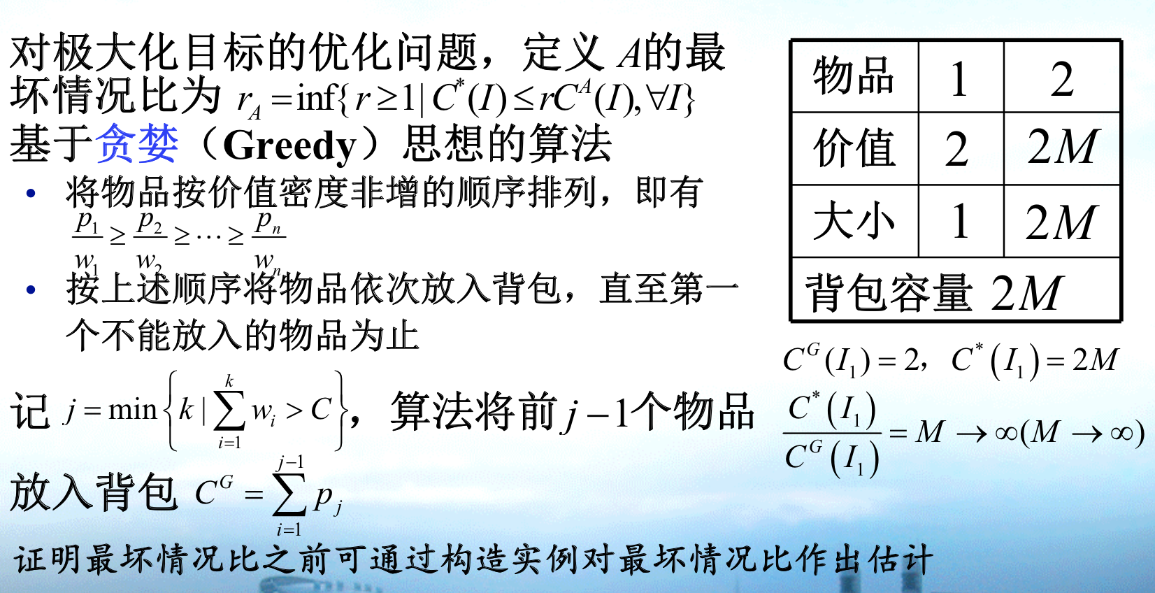
Note: the approximate ratio is \(\infty\), so we have to improve it
1.2.5. improved greedy
Algorithm: improving greedy method
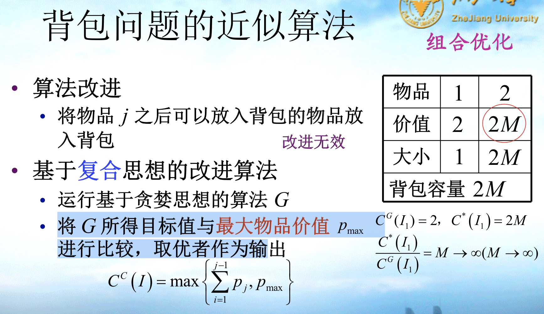
Qua: the approximate ratio is 2
Proof: using a upper bound (UB1)
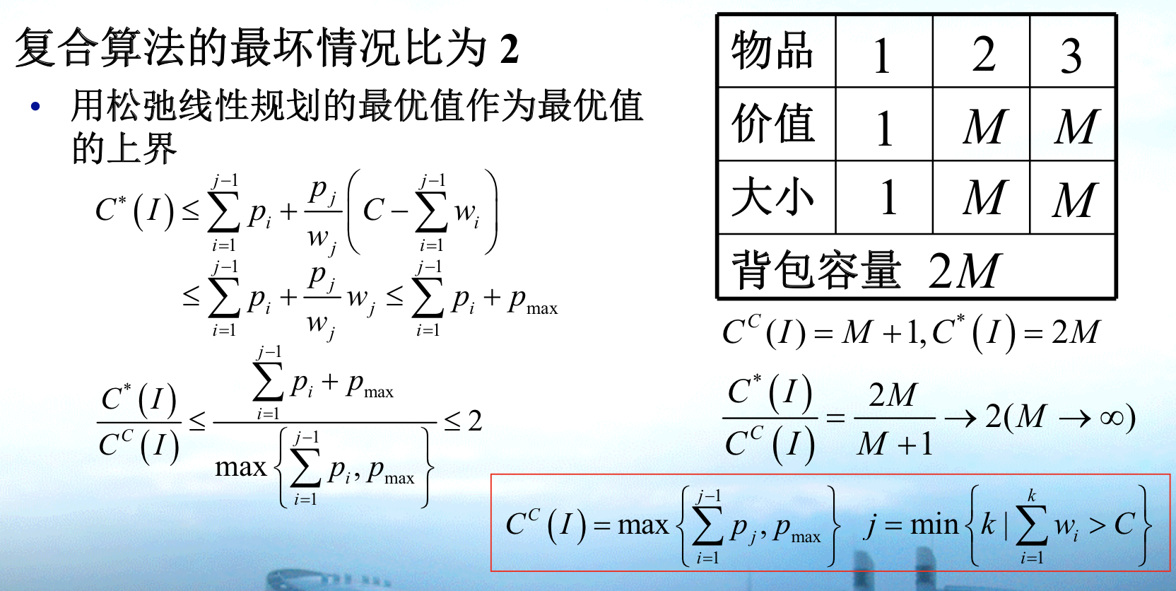
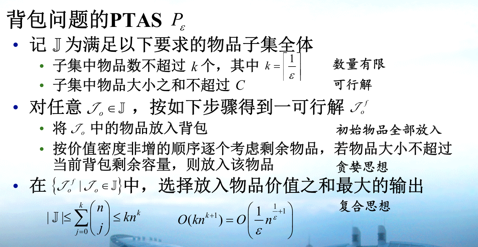
1.2.6. PTAS
Algorithm : PTAS
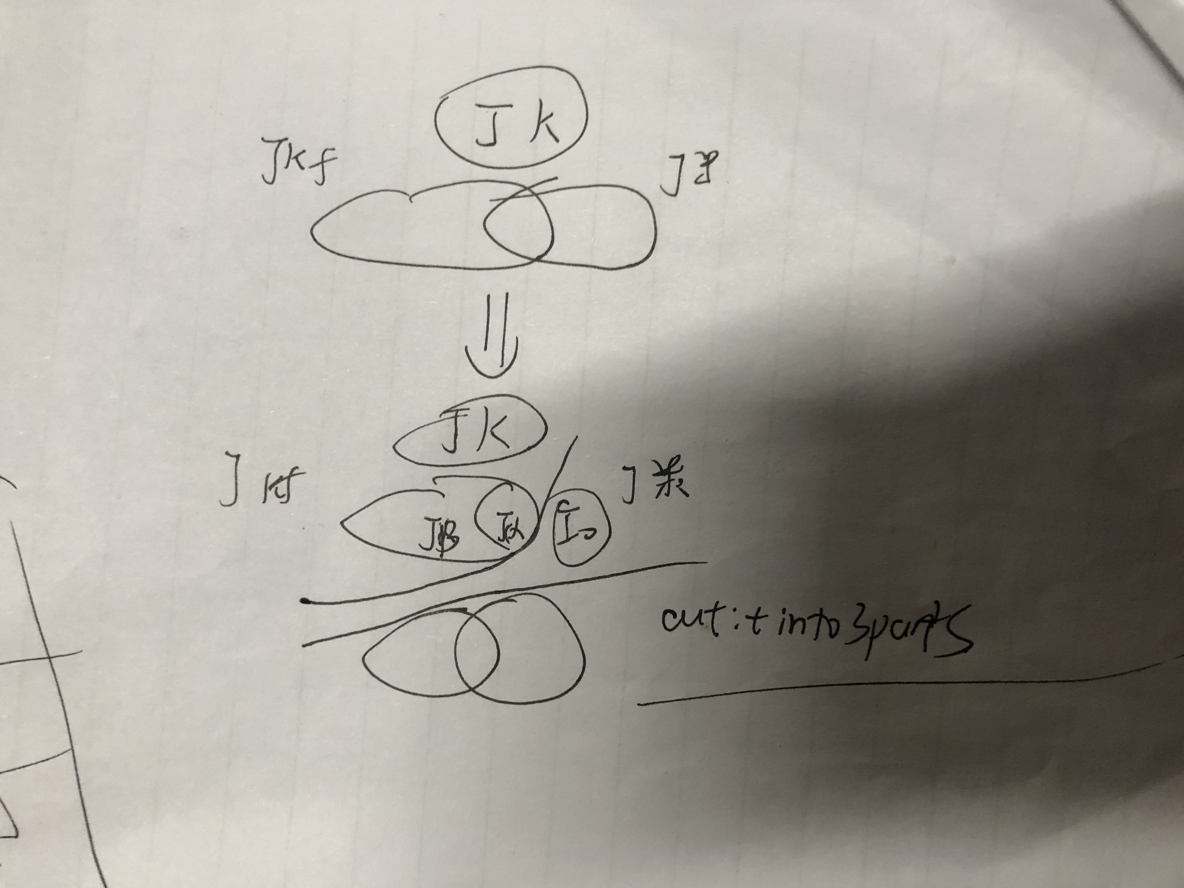
Usage: ensembling \(2^k\) possible solution together and output the best of them. 1) design a feasible bu t not optimal greedy solution 2) k is used to bound time & maximize capability of greedy solution.
Proof: separate the JK into 2 part by i0. the first part consist only intersection & jk itself, because no samples exists only in J* before i0. the second part consist of 3 part. This construction is done by introducing i0, have nothing to do with Jk algorithm(only Jk indicate that Ja+beta is not empty since i0 can't be the largest )
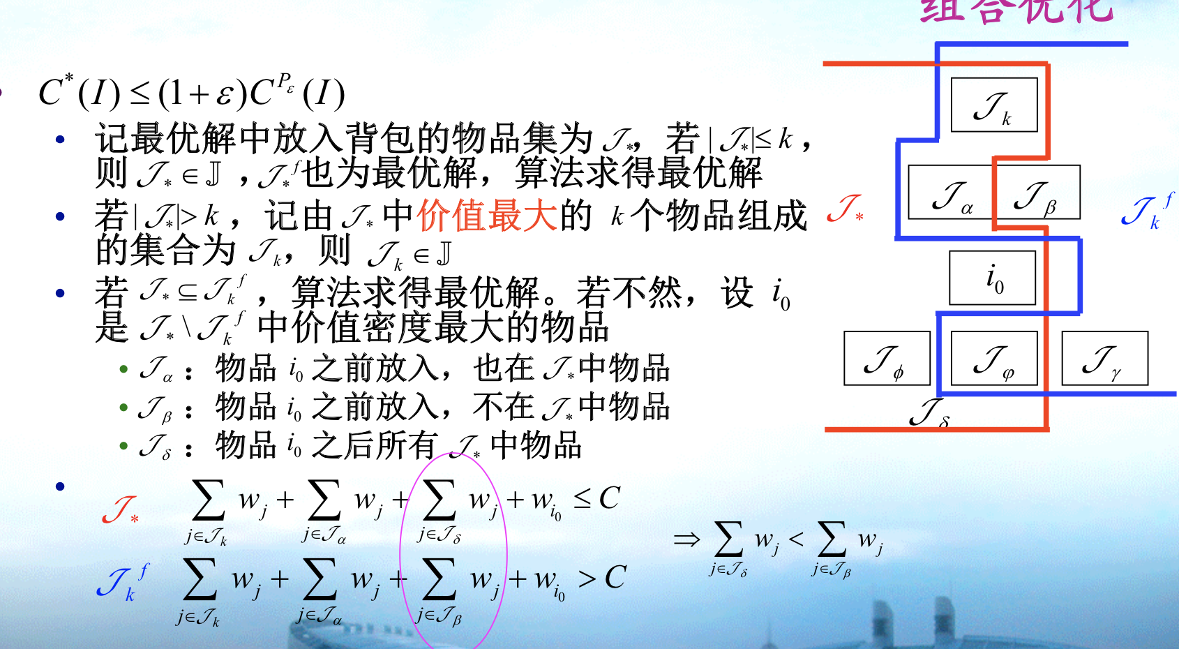
Note: this is a greedy solution. Key point of proof is Jkf have lower bound \(\alpha + \beta\), and use that lower bound with conditions provided by \(i_0\)(密度&重量), we can finally prove the point.
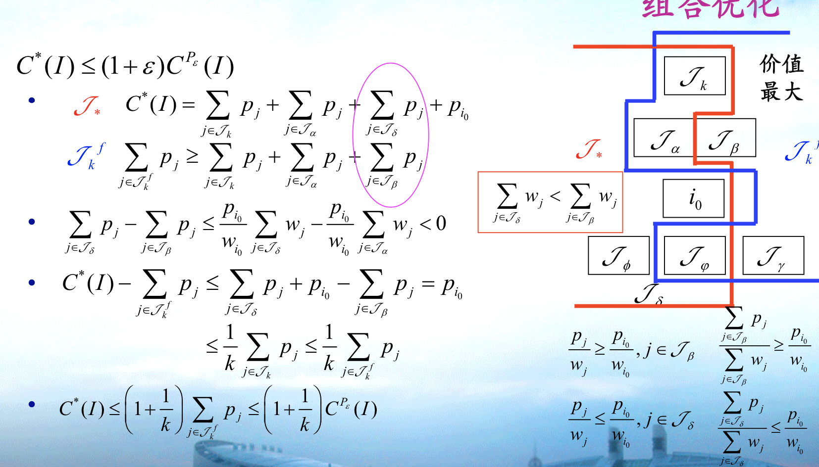
Note: fig
IMG_4922
1.2.7. FPTAS
Algorithm: FPTAS
Note: how to design a FPTAS => 1) design a unfeasible solution and make constraints 2) t is used to bound poly run time & reduce MAX of instance(maximize the capability of DP in another way by making it feasible).
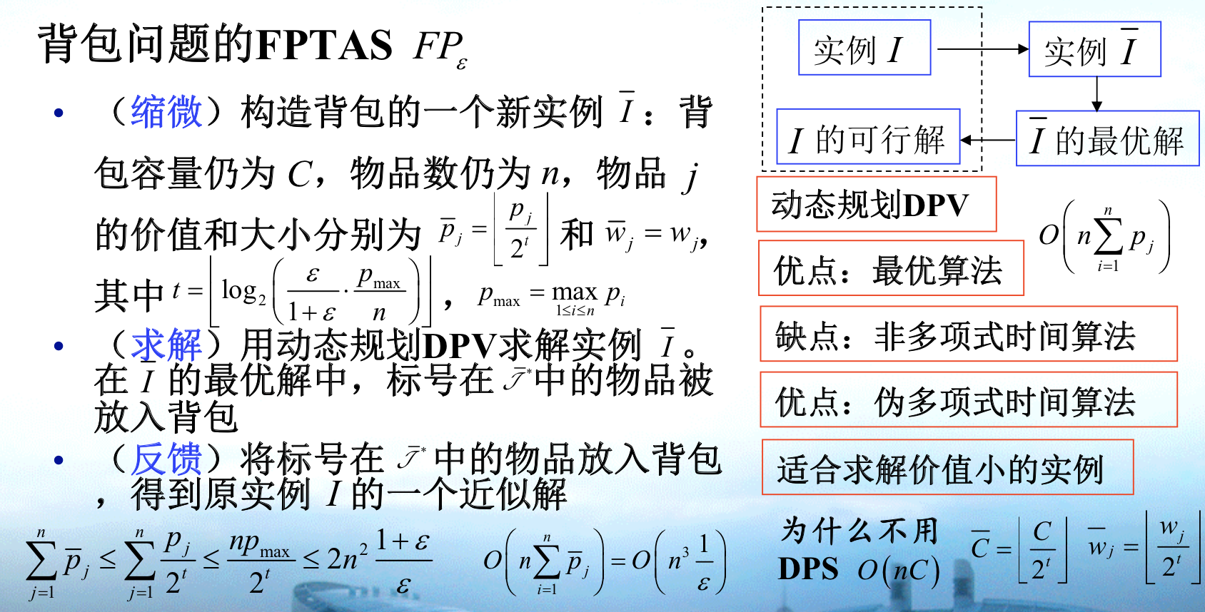
Proof:

Note: 从一个伪多项式算法出发,设计一个P缩微的实例。(之所以不放C,是因为可行性有可能改变)从这个实例出发,从左上到右上到右下到左下,右上右下都是天然下界。
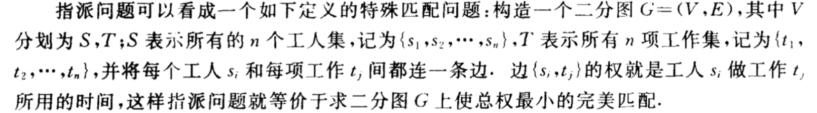
1.3. assignment problem
Def:assignment problem

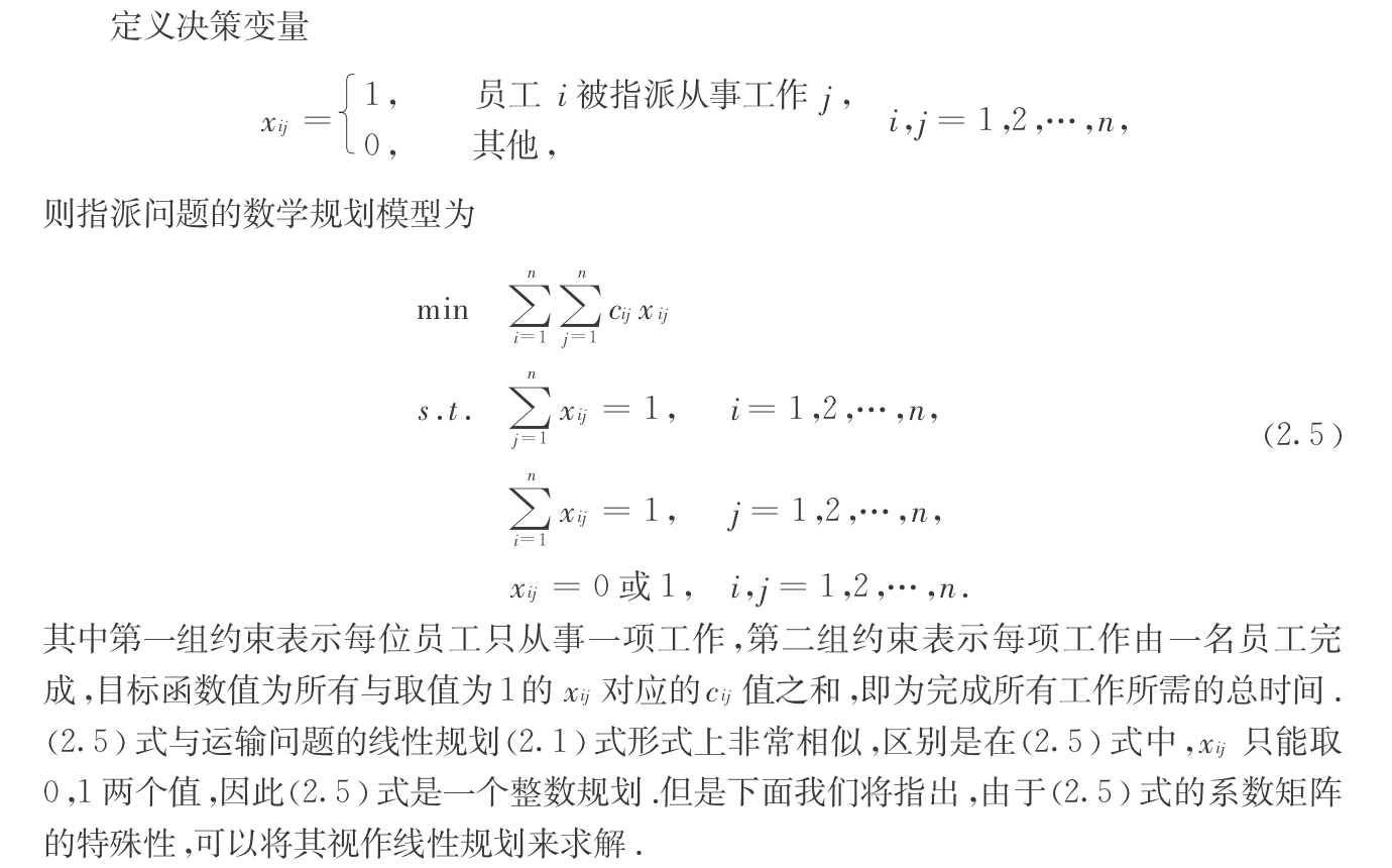
Note: standard form
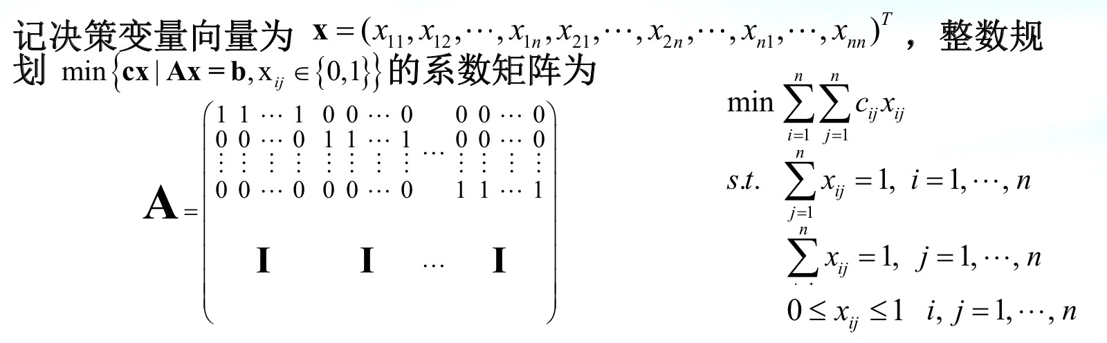
Qua: P( special kind of integer programming is poly solvable, NP-hard is defined when n->inf)
Qua: equivalent to Bipartite Matching
Qua: standardization, A is shown above, A is totally unimodular matrix
1.4. subset partition problem
Def: partition problem
desicion version

img opt version

img
1.5. product partition
Def: product partition problem
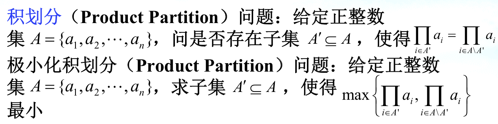
img Qua: NPC, have FPTAS

img
1.6. closest point
Def:
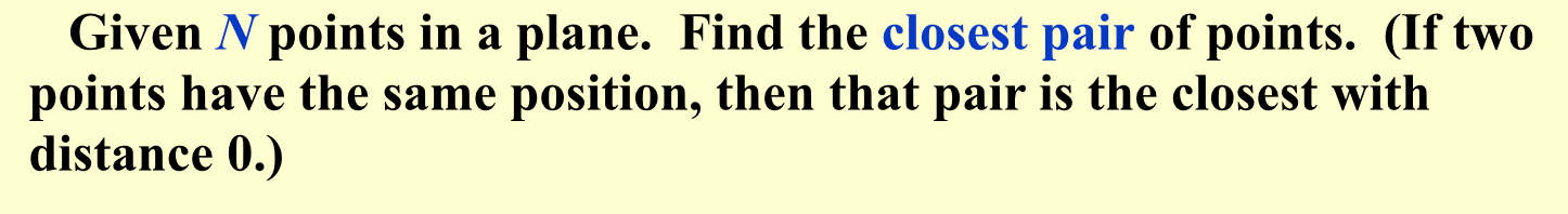
1.6.1. brutal
- Algorithm:
- Complexity: \(O(n^2)\)
1.6.2. divide & conquer
Algorithm:
https://blog.csdn.net/qq_22238021/article/details/78852337
- Complexity : \(O(nlogn)\)
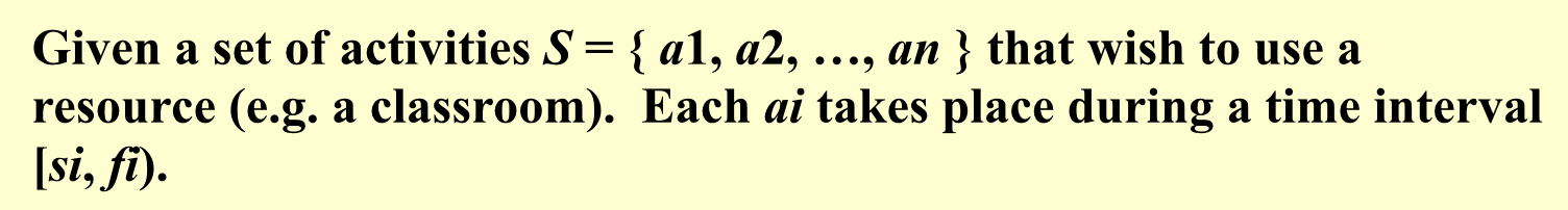
1.7. activity selection (max span)
Def:

1.7.1. dp
Algorithm: discretion \[ dp[i] = \max _{j=1->i-1} (dp[j]+span[i]) \text{ if j is compatible } \]
- Complexity : \(O(n^2)\)
1.8. activity selection (max size)
Def:
1.8.1. dp
Algorithm: discretion \[ dp[i] = \max _{j=1->i-1} (dp[j]+1) \text{ if j is compatible } \]
- Complexity : \(O(n^2)\)
1.8.2. dp2
Algorithm: discretion \[ dp[i] = binarySearch_j (dp[j]+1) \]
- Complexity : \(O(n logn)\)
1.8.3. greedy
Algorithm: greedy \[ dp[i] = dp[i-1]+1 \text{ if i is compatible } \\ \text{with max span of i-1} \]
- Complexity : \(O(n)\)
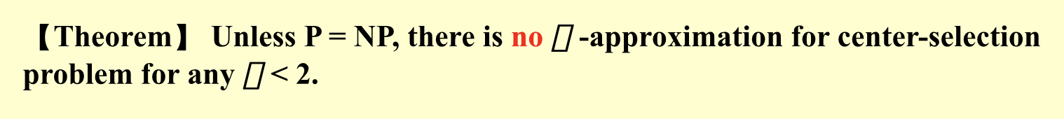
1.9. k-center
Def:
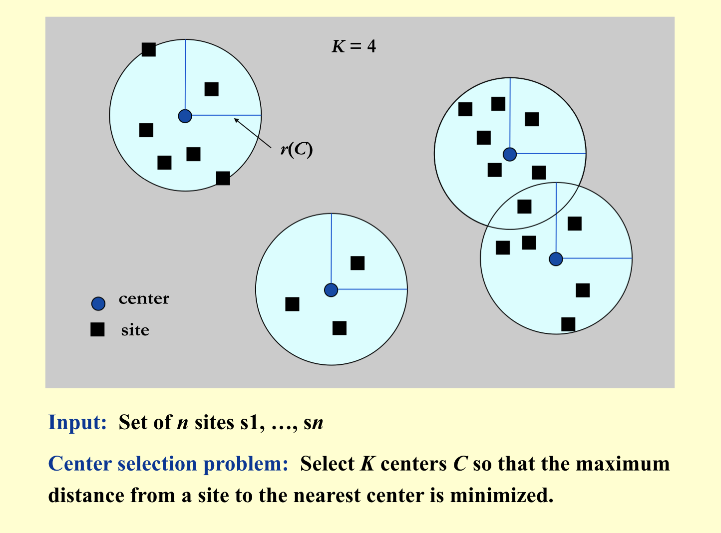
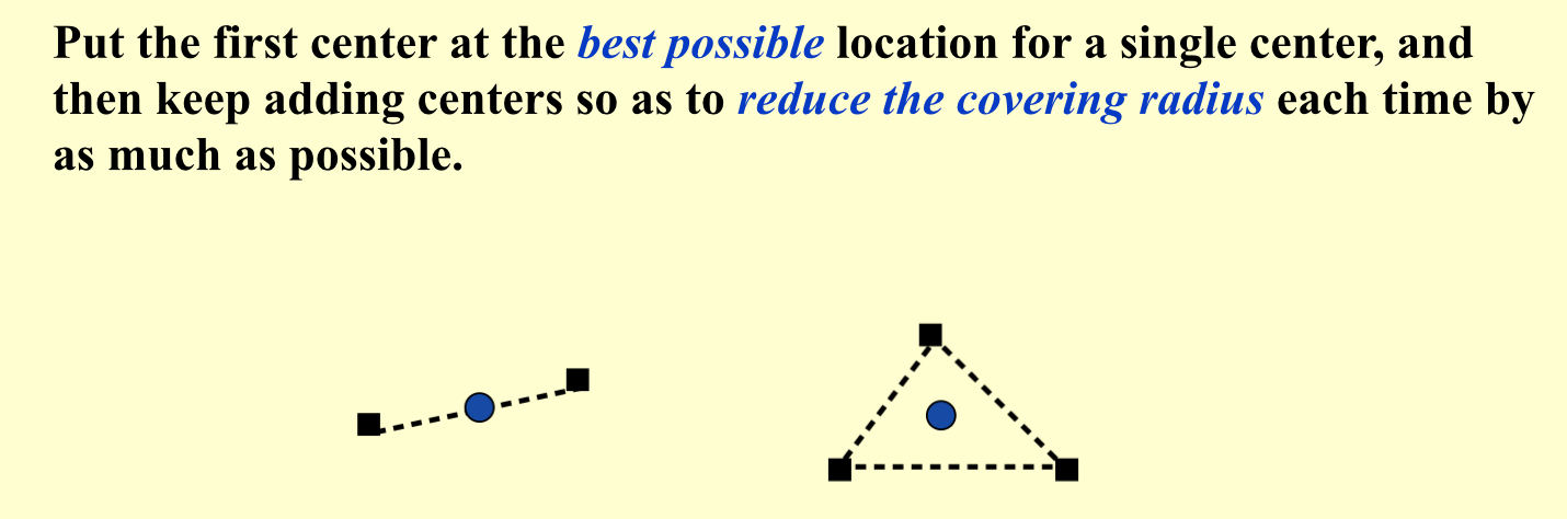
1.9.1. greedy1
Algorithm:
1.9.2. greedy2
Algorithm:
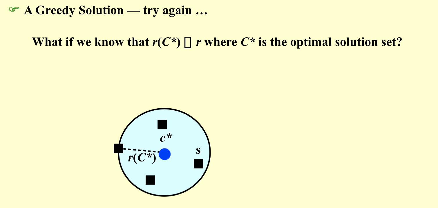
Qua: ratio = 2
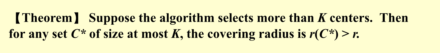
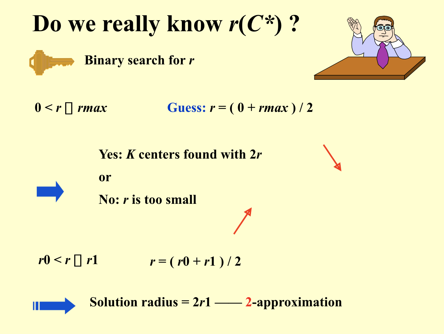
Qua: ratio \(>=\) 2
1.10. hiring problem
Def:
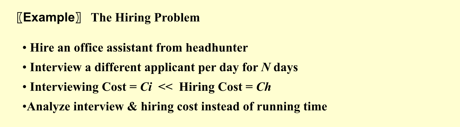
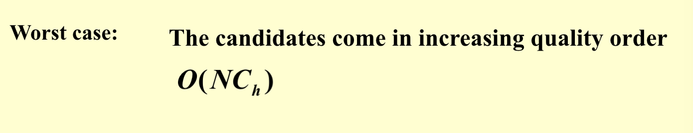
1.10.1. brutal
Algorithm:
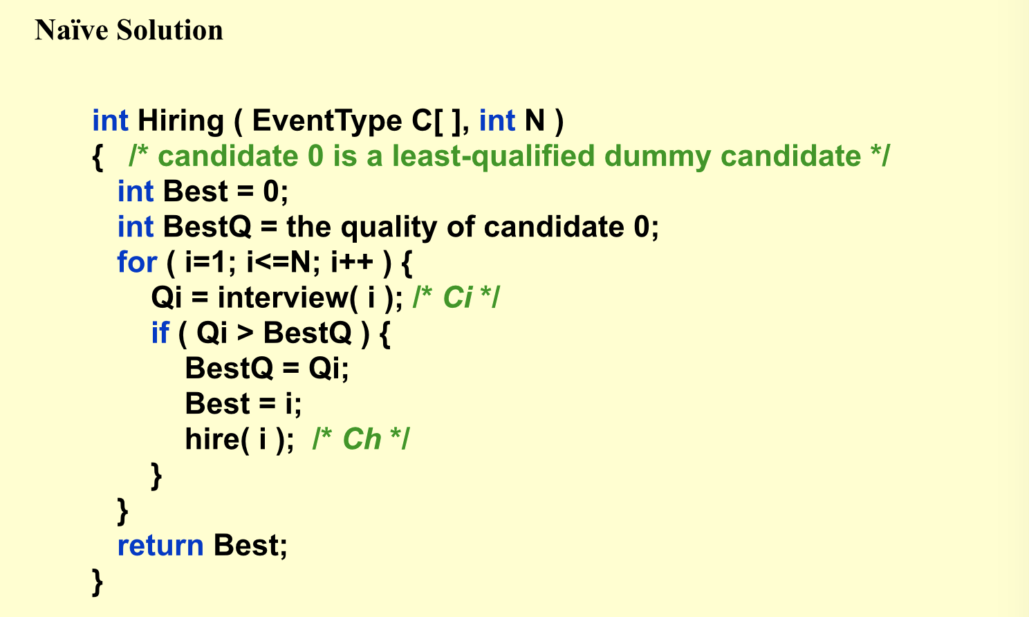
Qua :
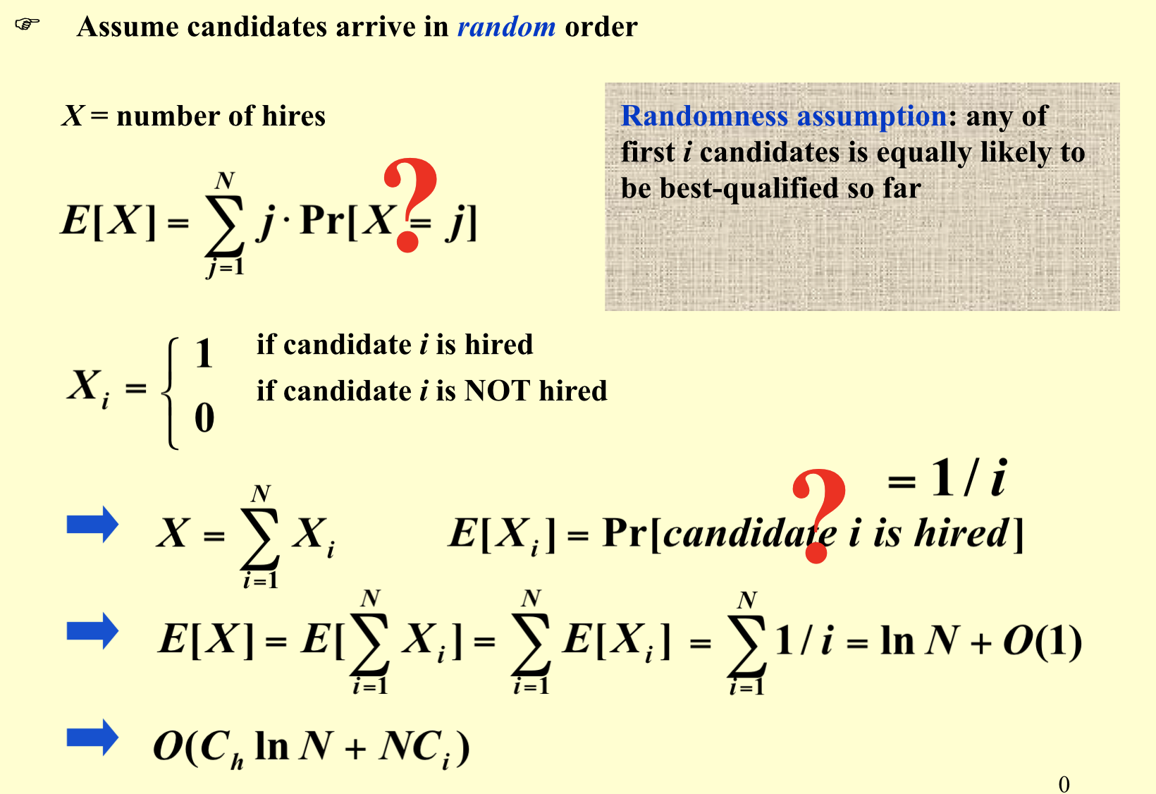
1.10.2. randomize
Algorithm:
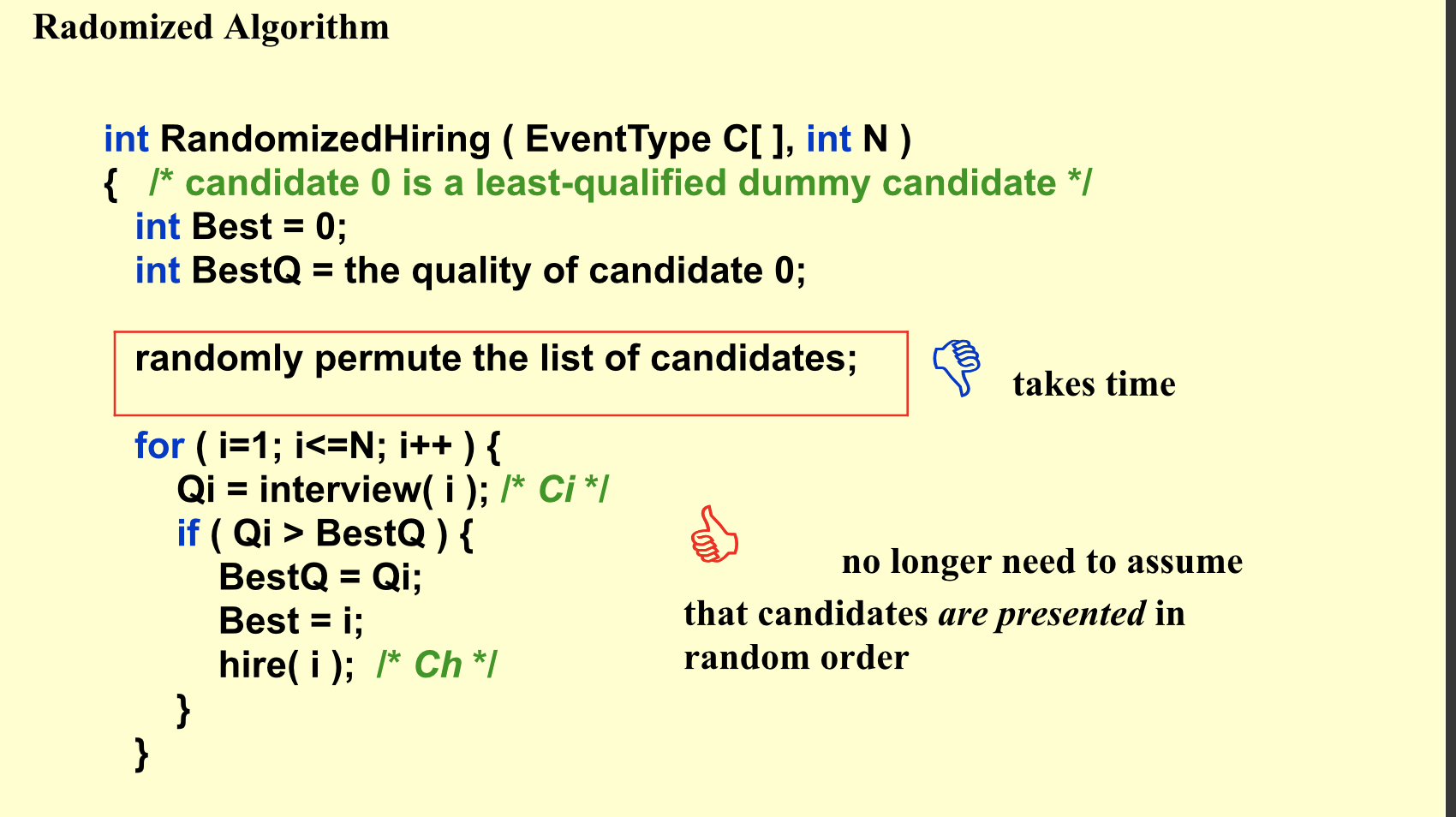
Qua:
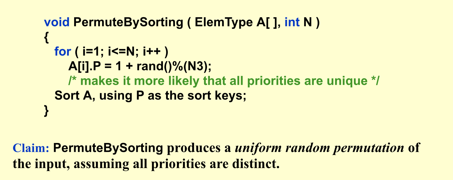
1.11. permutation
Def:

1.11.1. randomize
Algorithm:
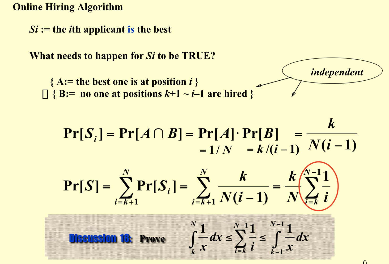
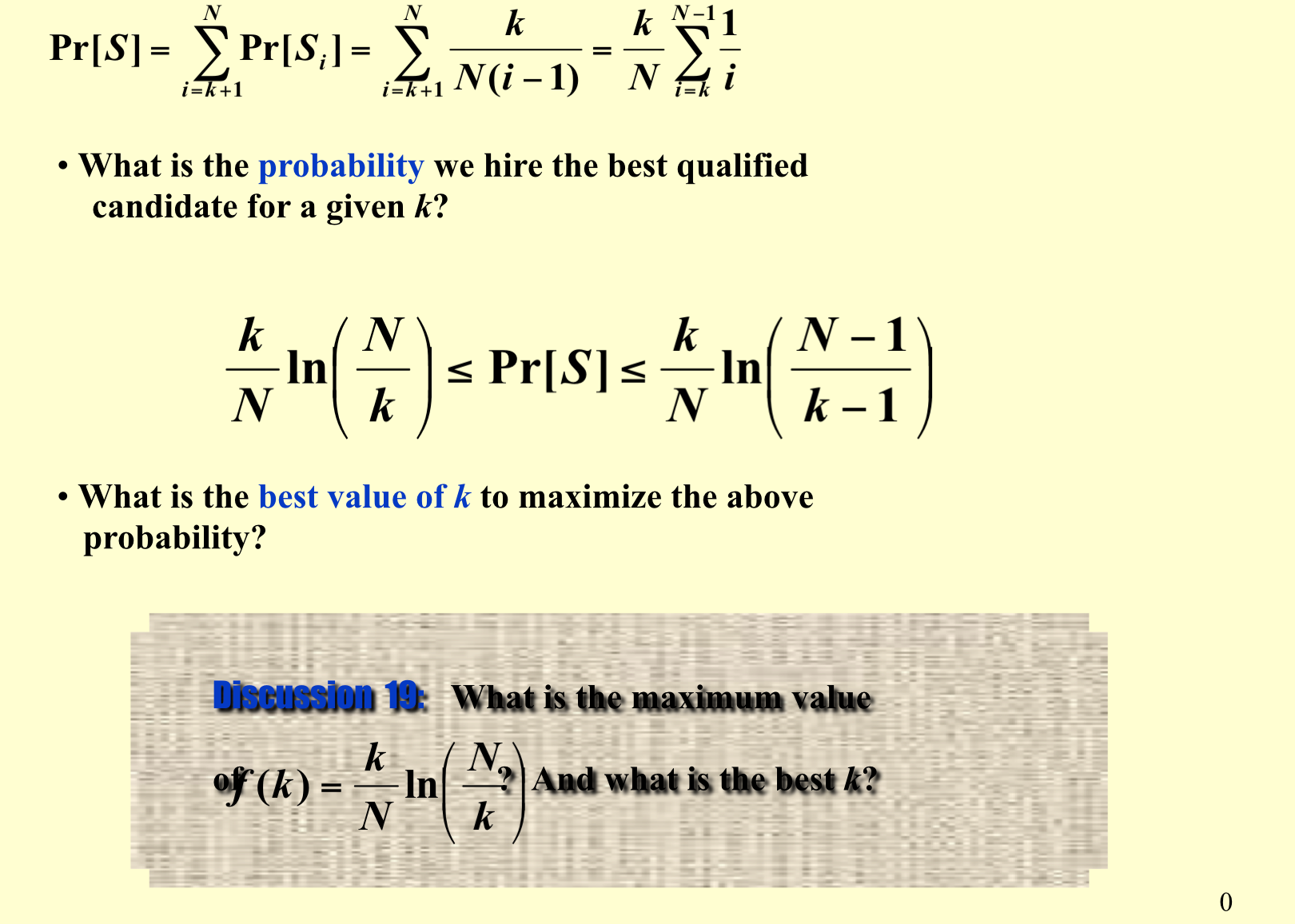
1.12. online hiring
Def:
1.13. scheduling
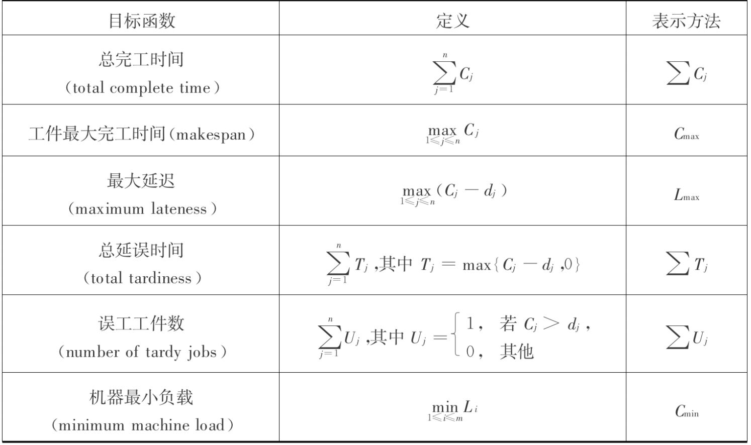
Def: scheduling problem
Usage: representing scheduling problem in 3 elements


Def: machine env ( \(\alpha\) )
Example: possible example of machine environment, note that parallel have no bounds on machine sequence, it's more like to make things more equal. And shop have bounds on sequences and shit have to be on multiple machines, it's more complicated.
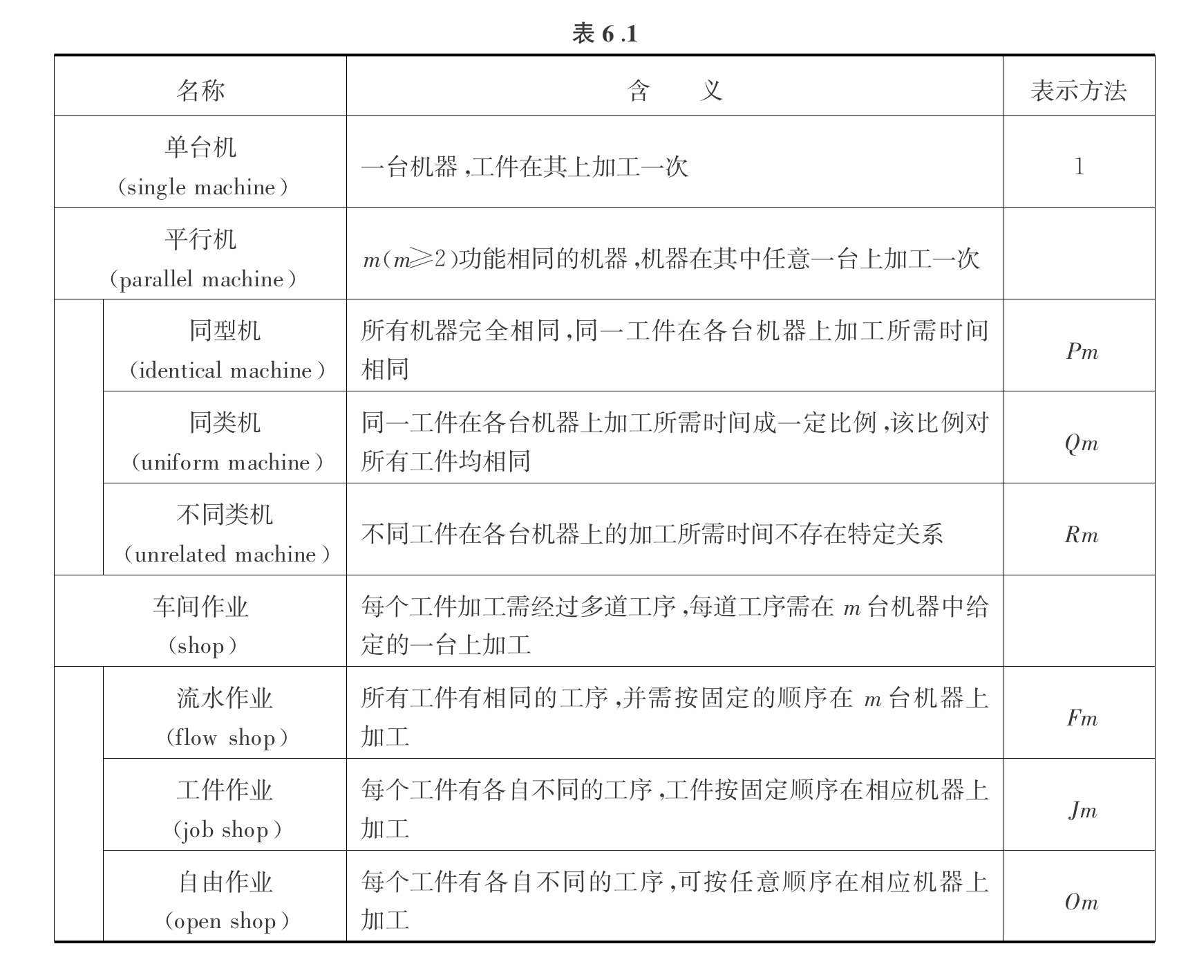
Note: mixed & hybrid
Def: job characteristic ( \(\beta\) )
Note: more constraint
Def: loss function ( \(\gamma\) )
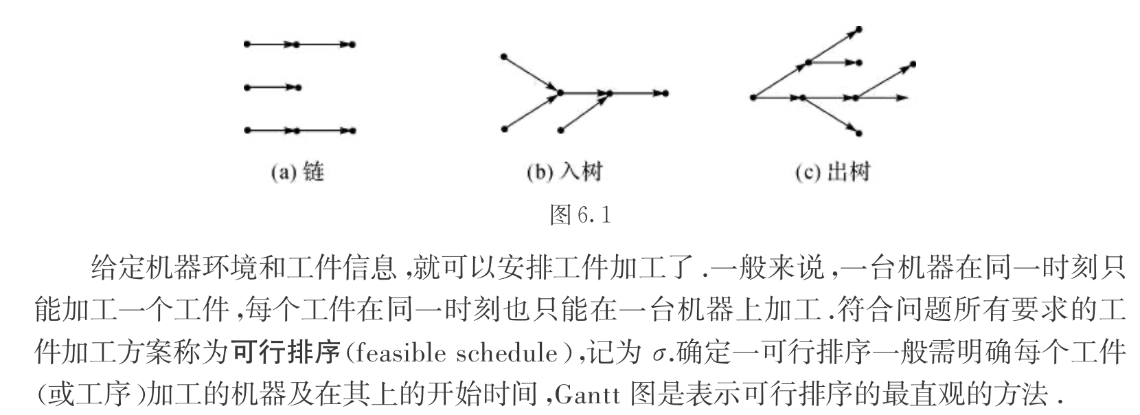
Def: gatt diagram
Usage: representing a possible solution
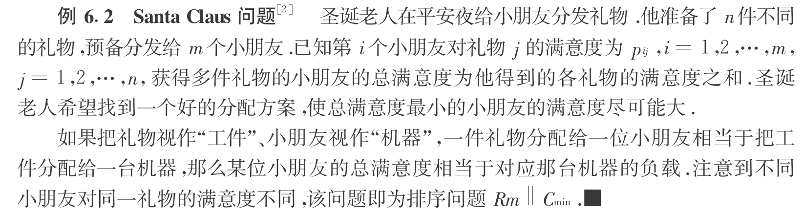
Example: Santa problem
Usage: the simpliest scheduling problem ( without precedence )
Example: parodox of scheduling problem
Usage: the cons for greedy algorithms: decrease job time & increase machine number will not necessarily yield better result.
P175
1.13.0.1. P1 Cj, Cmax, L1max, Tj, Uj
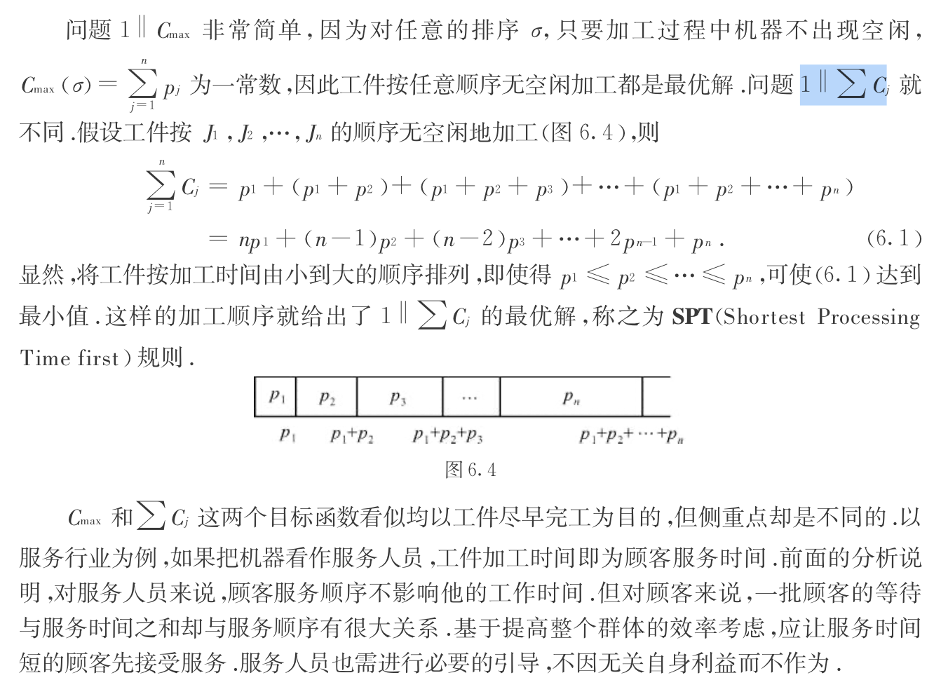
1.13.0.1.1. \(C_{max}\) or \(\sum_{n=1}^{\infty} C_j\)
Def: \(C_{max}\) or \(\sum_{n=1}^{\infty} C_j\)
Algorithm: for \(\sum_{n=1}^{\infty} C_j\): SPT
Algorithm: weighed sum cj \(\sum_{j=1}^{n} w_jc_j\)
Note:
0.0) \(\sum_{n=1}^{\infty} wjcj = (w_1+...w_n)p1 + ...\)
1.0) when n = 2, get solution \(w_2p_1\) vs \(w_1p_2\)
2.0) when n > 2, insights from n =2, sort \(\frac{pj}{wj}\)
Proof:
1.0) swapping 2 element i,j => contradiction,
1.1) set i - j =-1 to make it easier.( this step is important since we only get information from i and j)
Algorithm: weighed functional sum of cj : \(\sum_{n=1}^{\infty} w_jg(c_j)\)
Qua; when g is convex: worst ratio = sup ...
Qua: when g is 分段linear: NPC
Qua: when g is \(x ^{\beta}\) => i <g j & i <l j
1.13.0.1.2. L1max, Tj, Uj
Def: one machine problem: \(L_{max}\) is the maximum of delay time. \(\sum_{n=1}^{\infty} U_j\) is the total delayed objects. $ _{n=1}^{} T_j$ is the added delayed time.

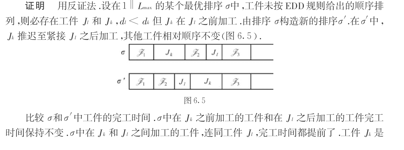
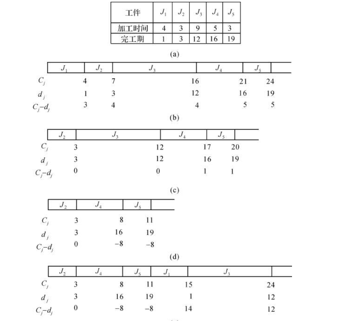
Algorithm: for \(L_{max}\): EDD

Proof: By contradiction. Note that we only need to prove \(L_{max}\) is not increasing, and only k, j, i changes in the \(\sigma'\) solution and everyone of them are bounded by the max($$) of the original.
Algorithm: for \(\sum_{n=1}^{\infty} U_j\) : Moore-Hodgeson(EDD improve)

Note: example of Moore-Hodgeson
Algorithm: for \(\sum_{n=1}^{\infty} T_j\)
Note: no resting time
Qua: => exist pseudo - p algo
Qua: => exist FPTAS
Qua: => NP-C
Algorithm: another loss function where we want "JUST IN TIME" : \(\sum_{n=1}^{\infty} T_j +E_j\) where \(Ej= max(d_j-c_j, 0)\)
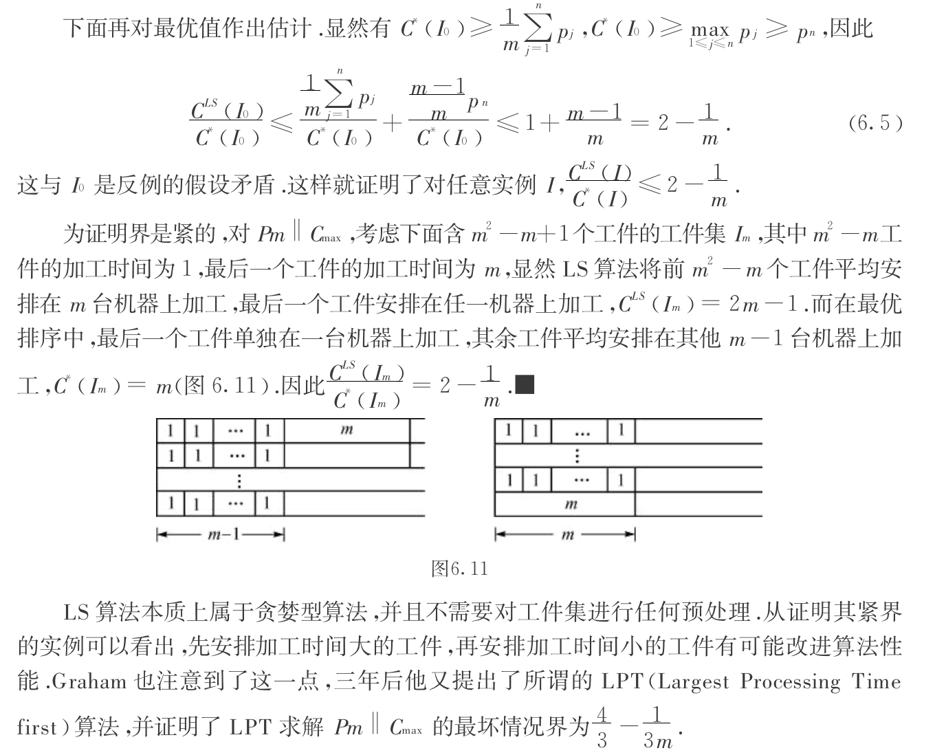
1.13.0.2. Pm Cmax, Cmin
Def: multi-machine problem Pm
Note: Pm and P difference: whether m is a given input(P) or constant(Pm), the consequence of this is that when Pseudo-P algorithm in Pm is O(P^m), it is exponential in P since m is input.

Qua: lower bound for \(C_{max}\) \[ C_{max}\geq \sum_{i=1}^{n}p_i /m \\ C_{max} \geq \max \limits_{i=[1,n]} pi \]
Qua: => NP-hard

Proof: obvious
from 2 to Pm|| ..: adding p-2 dummy node with cj = C
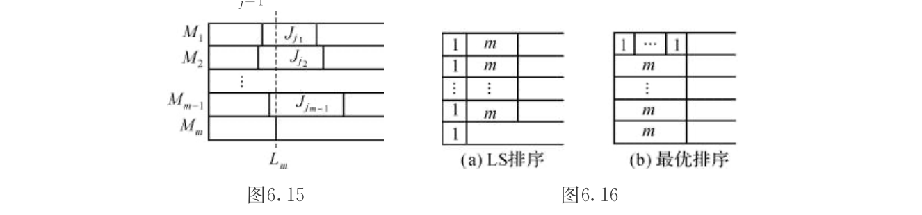
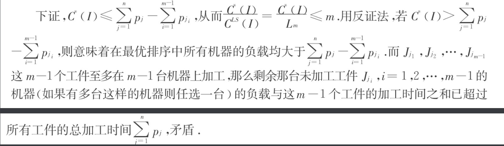
Algorithm: LS
Note: the most important thing is when \(j_i\) is placed on m machine, then other machines are not ready. \(\sum_{i=1}^{n-1} p_i \geq s_nm\)

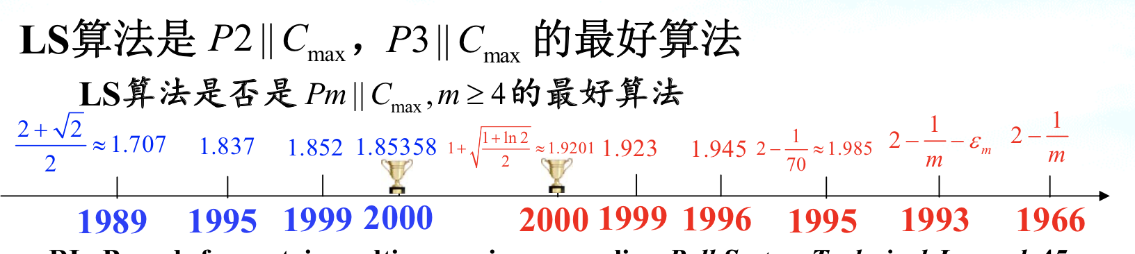
Qua: worst ratio \(=\) 2- 1/m

Proof: By contrast & minimal conter example: extra information by introducing minimal counterexample instead of counterexample.
1)first prove that Jn determine max span: exactly why we introduce minimal conterexample, this is intuitive since you can always cut the final element if the final element does not decide max span.
which means \(Cls(I0) = s_n + p_n\)
2)then prove by lower bound of C*
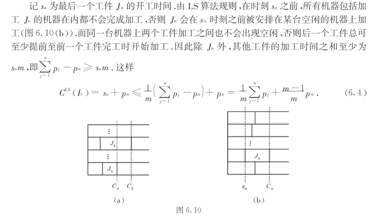
3)tightness prove: find an example that have 2 - 1/m: consider LS's con, LS can fill in small items to small which makes things worse.
Note:
Algorithm: LPT(sorted LS)
Insight: from the worst case of above, that we do from large -> small this time.
Note: note that the additional information is \(C^*(I) <3p_n\) => each lane has at most 2 items, since \(p_n\) is the smallest item

Qua: worst ratio

Proof:
1)LPT can exclude \(C^*(I) < 3 p_n\), that if it suffice, at most 2 items is on each lane in optimal solution. So that leaves us \(C^*(I) \geq 3 p_n\)
2)By construct, construct a LPT solution by transforming a optimal solution( one on one relationship between LPT with some optimal).
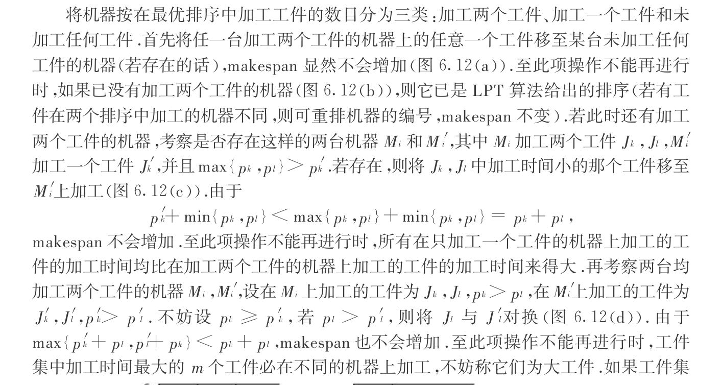
3)tightness proof
Def: Pm||Cmin (maximization problem)
Algorithm: LS
Note: LS gives us \(L_i- p_{j_i} \leq L_m\)
Qua: worst ratio = m

Proof:
1)prove ratio $ $ m
1.1) By provided condition: first prove lower bound for Cls: Lm
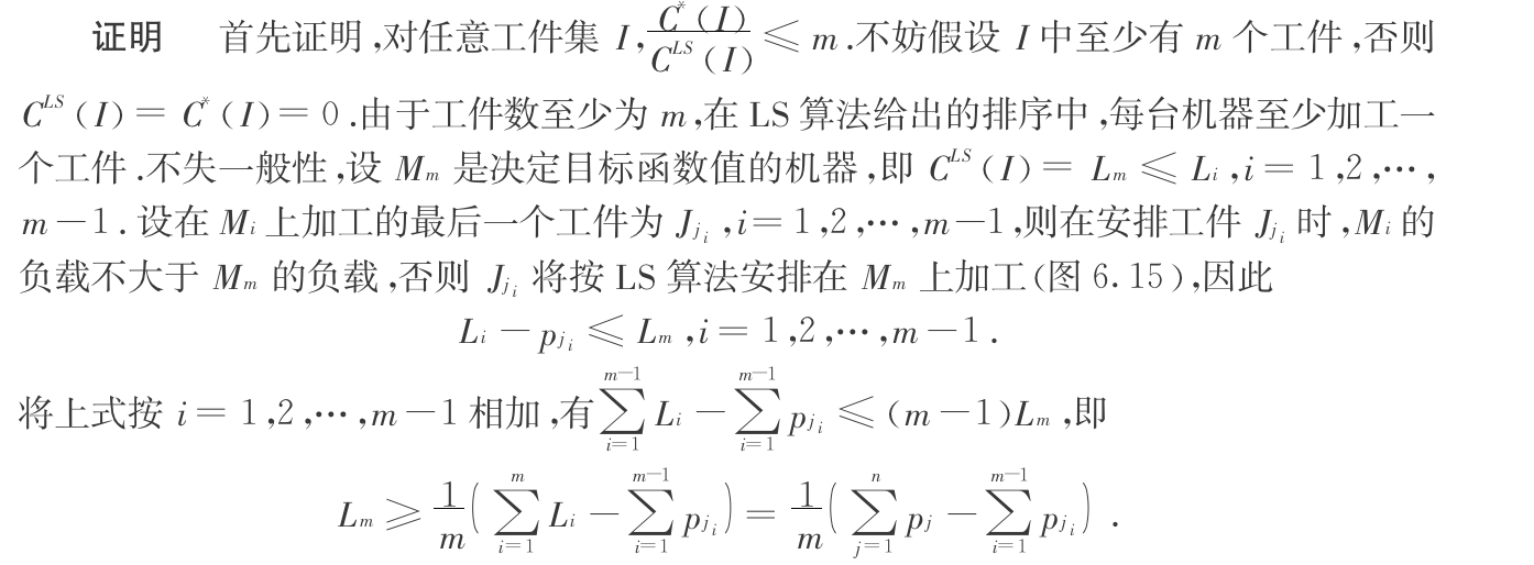
1.2) By contradiction, second prove upper bound for C*
2)ratio \(\geq\) m, same as LS Cmax, but swap 1 & m
Algorithm: LST
- Qua: worst ratio = \(\frac{4m-2}{3m-1}\)
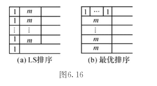
Qua: for every instance, there's not always a scheduling that satisty both optimal for Cmax & Cmin. But is there an algorithm such that ratio_min < \(\alpha\) and ratio_max < \(\beta\) ?
1.13.0.3. P Cmax
Def: P||Cmax
Qua: strong NP-hard
Proof: 3-partition $ _p $ P||Cmax
Note: Pm||Cmax can not use this reduction since m in Pm is a constant .
1.13.0.4. F2 Cmax
Def: F2 Cmax

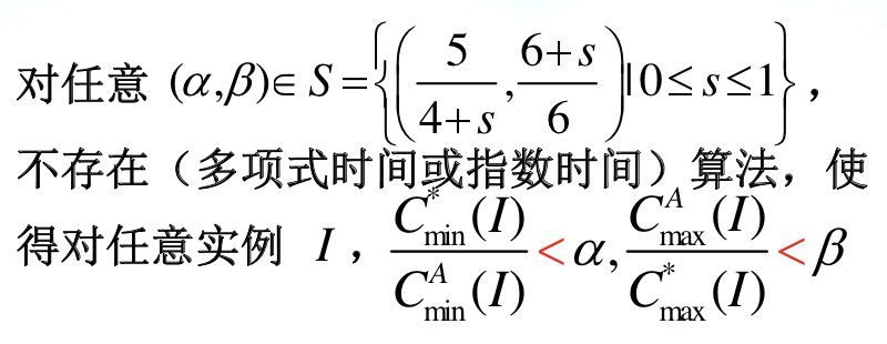
Algorithm: Johnson
Note: why sort the second array?
Note: fig
1.13.0.5. F3 Cmax
Def:
Qua: worst ratio <= 5/3 or 3/2

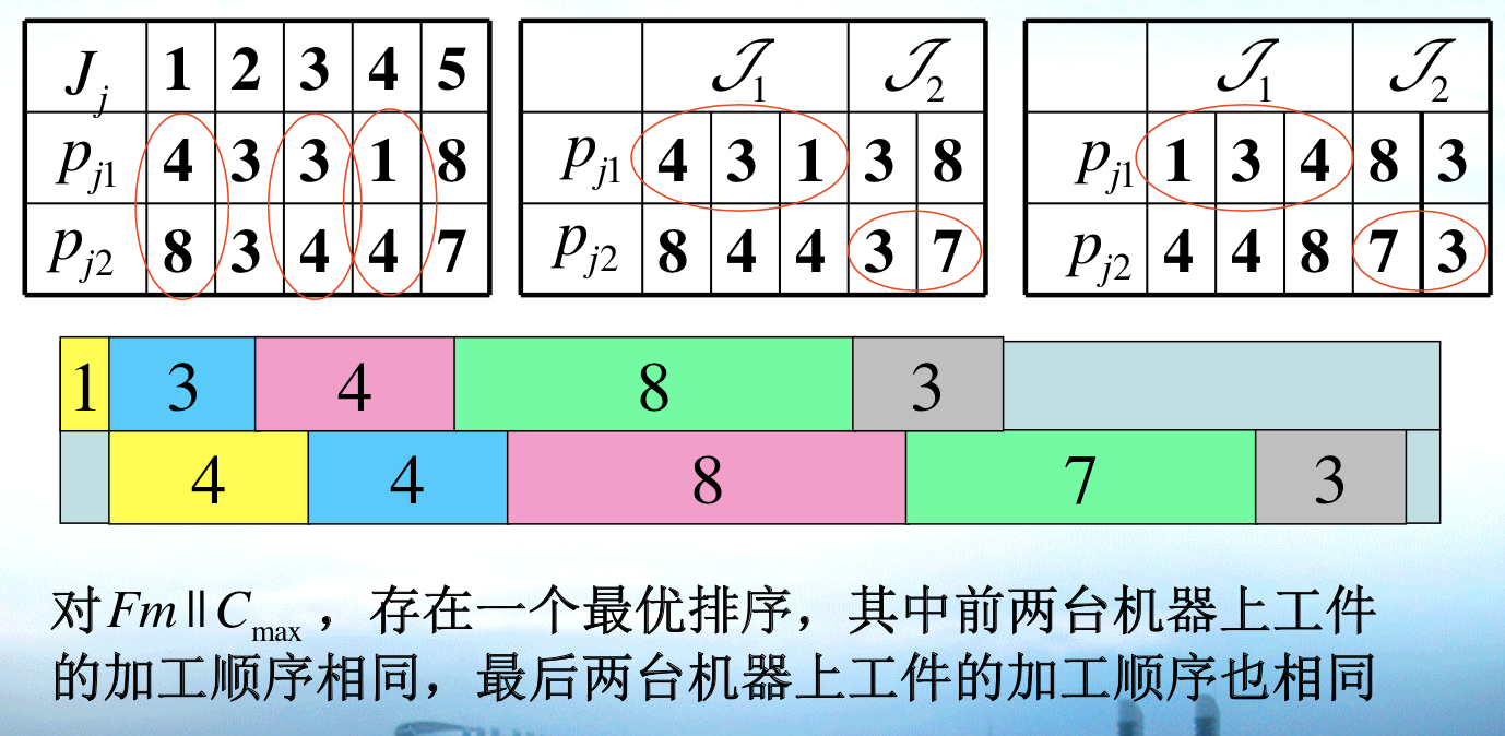
1.13.0.6. Fm Cmax
Def:
Qua: possible lower / upper bound
Note: LB = max{dilation, congestion}. dilation = $max {j=1}^{n}pji $ , congestion = $max {i=1}^{m} pji $
dilation is the max sum of item since every item have to finish all routine, congestion is the max sum of machine since machine have to finish given work.
Qua: exists PTAS

Qua: worst ratio > 5/4

Qua: worst ratio <=2 / log....
1.13.0.7. O2 Cmax
Def: O2 Cmax

Algorithm: johnson
Qua: this is a feasible & optimal solution
Proof:
1)first prove that separatly they are feasible

2)then we combine those 2 and prove that they are still feasible
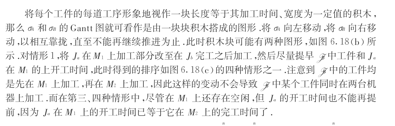
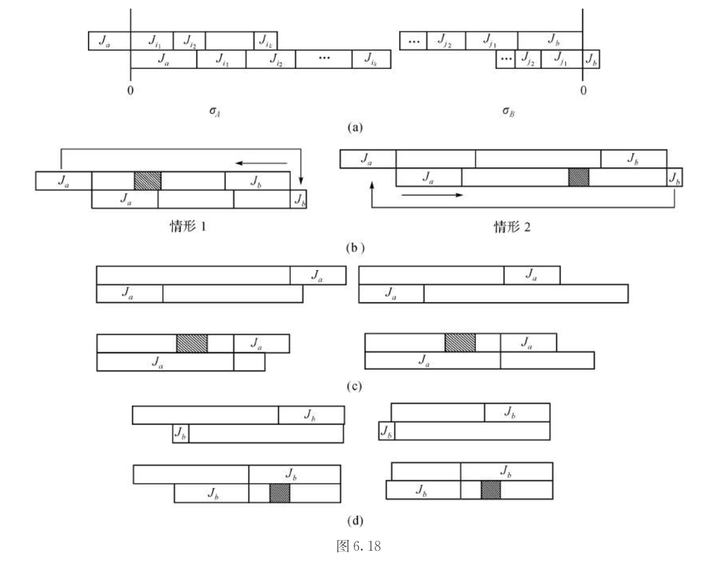
3)By equals lower bound(for min): prove optimal
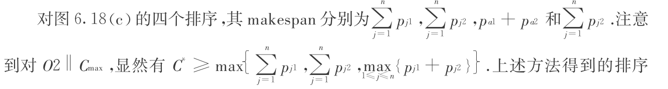
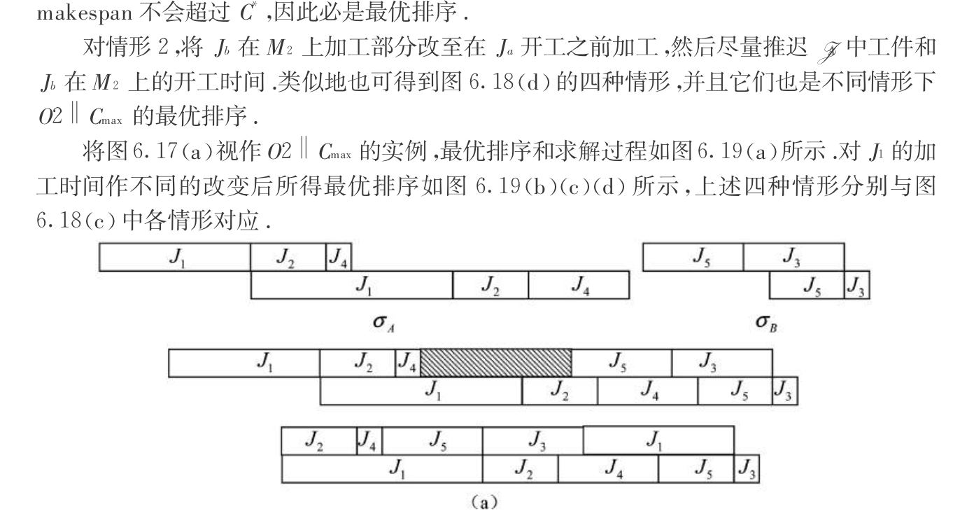
traverse through all possible solutions and get solution = lowerbound.
1.13.0.8. O3 Cmax
Def:
Qua:

1.13.0.9. Om Cmax
Def:
Qua: exist FPTAS

Qua: worst ratio

1.13.0.10. Jm Cmax
Def:
Qua: worst ratio >= ....

1.13.0.11. Rm Cmax(hw)
Def: ...
Qua: lb for some algo = m
Proof: \(\leq m\) => ...
\(\geq m\) => 1 and 1 + \(\epsilon\)
Qua: online lb
Proof: (1,1) => (1,2) & (2,1)
1.14. bin-packing
Def: bin-packing problem

Qua: worst ratio \(\geq\) 1.5

Proof: By gap tech, bin\(\leq p\) partition
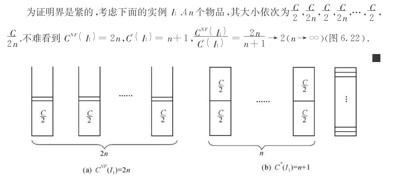
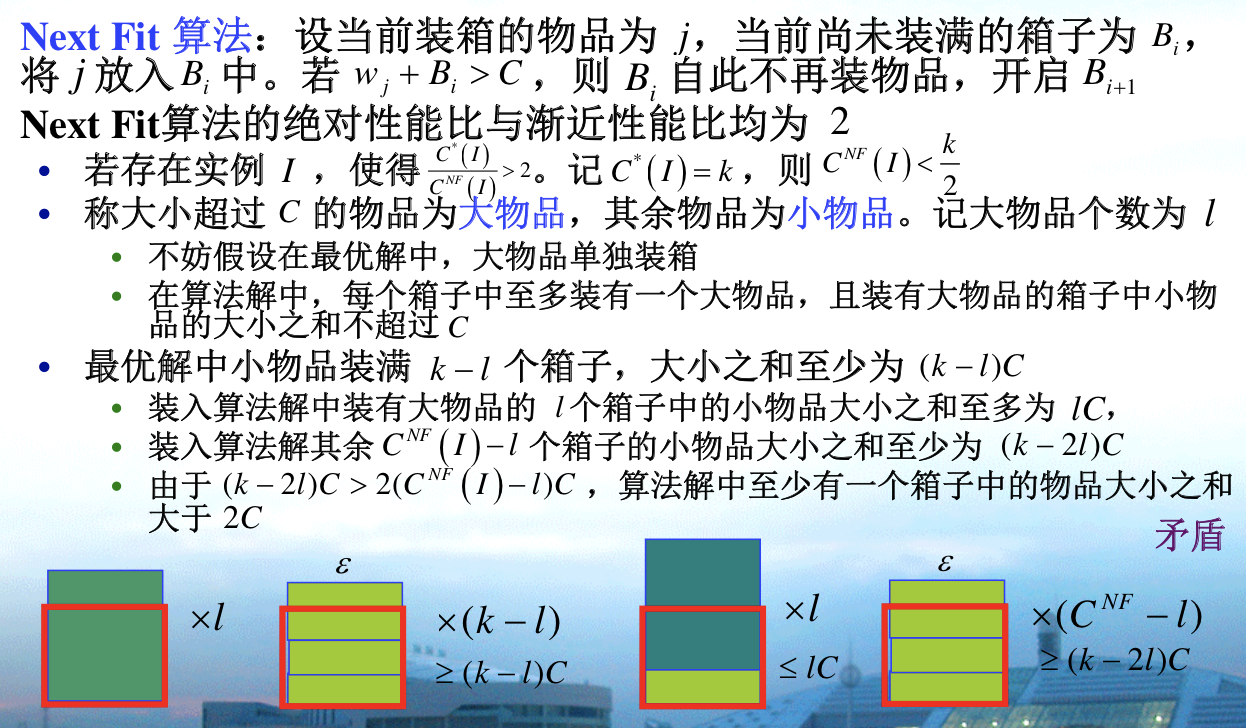
1.14.0.1. next fit
Algorithm: next fit ( influenced by sequence )
Note: fit => fill; not fit => new box
Qua: worst ratio = 2
Proof:
1)By constrast, ratio \(\leq\) 2 ( from local => global )
2)ratio \(\geq\) 2, consider to let every box as empty as possible(at least C/2)
1.14.1. greedy: first fit
Algorithm: first fit
Note: 1 => j, fill the first fit or new bin


Qua: worst ratio = 1.7
Proof: proof is crazy, same idea: make boxes as empty as possible.
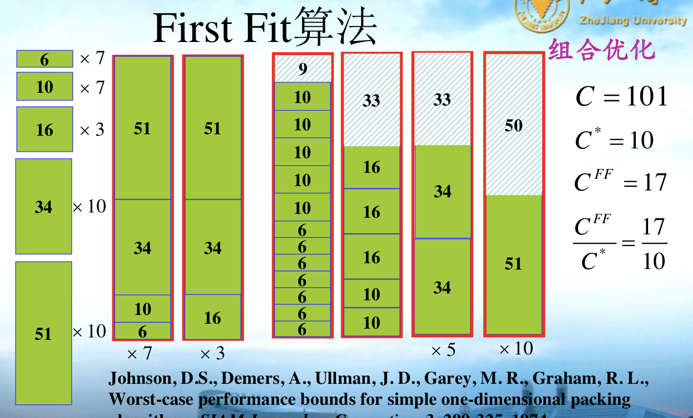
1.14.2. greedy: first fit decreasing
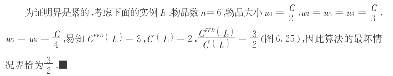
Algorithm: first fit decreasing (FFD)
Note: sort non-increasing + first fit, FFD provide sorting sequence which is very important.

Qua: worst ratio = 1.5
Proof: want to get upperbound for l => upperbound for pj and j
1)prove ratio \(\leq\) 1.5
1.1) By given FFD, prove upperbound for \(w_j\)

1.2) By given FF, prove upperbound for j

1.3) By, upperbound: finally prove it.
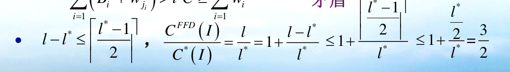
2)By l-l* lowerbound, which means trying hard to make them close: prove ratio \(\geq\) 1.5
Note: relaxation can be made => \(p_j \leq C/2\) will suffice ( see slides )
1.15. online ski-rental
Def: ski-rental problem
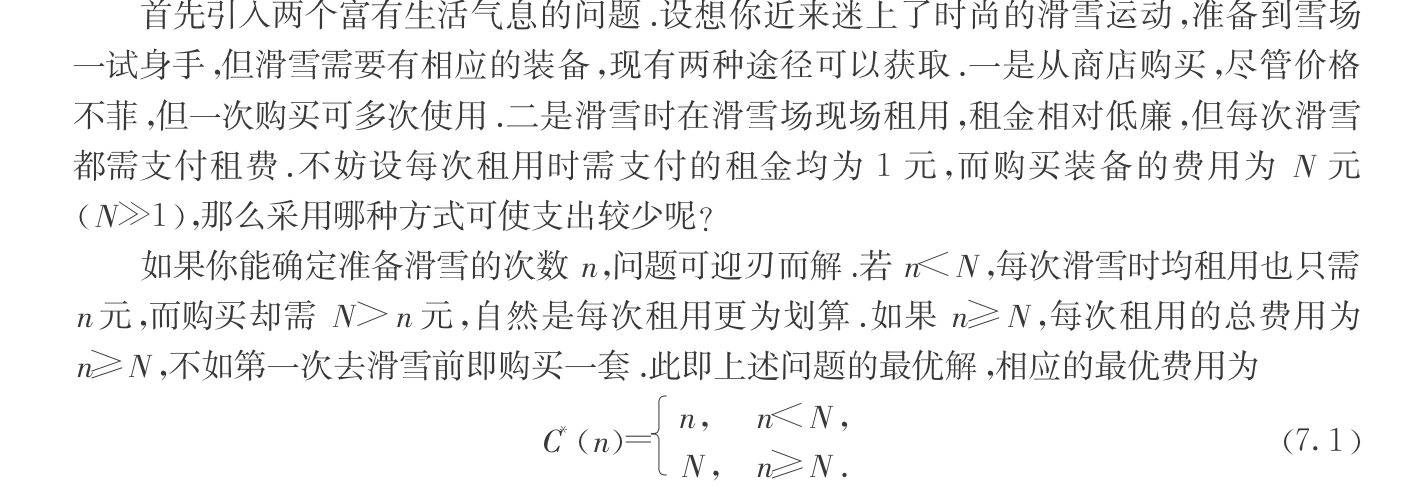
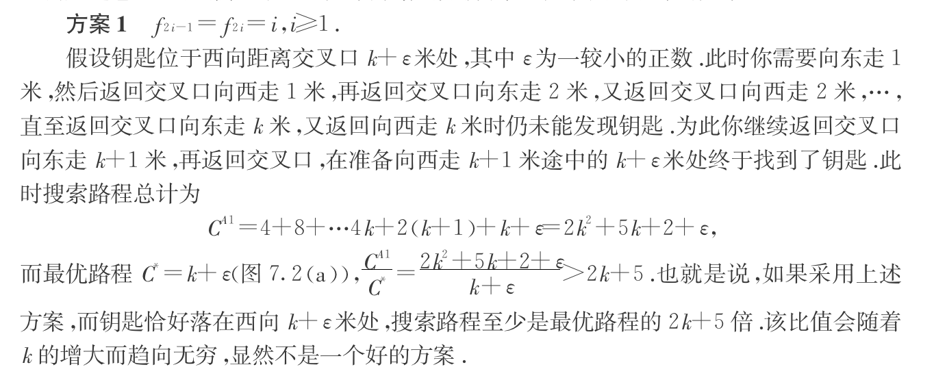
1.15.1. greedy: strat-N
Algorithm: strat-N

Qua: lb \(\leq\) 2

Qua: strat-N is the best of strat-K
Note: draw a diagram with ratio on instance level

1.16. bin-covering
Def: bin-covering problem

1.16.1. greedy: next fit
Algorithm: NF
Proof: By contraction.
Qua: ratio \(\geq\) 2

1.17. online searching
Def: online searching 1D
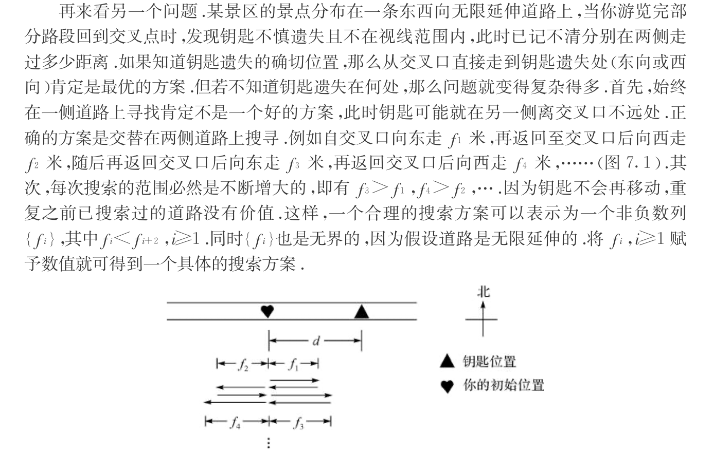
1.17.1. greedy: linear space
Algorithm: linear pace
Note: linear pace 2
1.17.2. greedy: exp space
Algorithm: exp pace
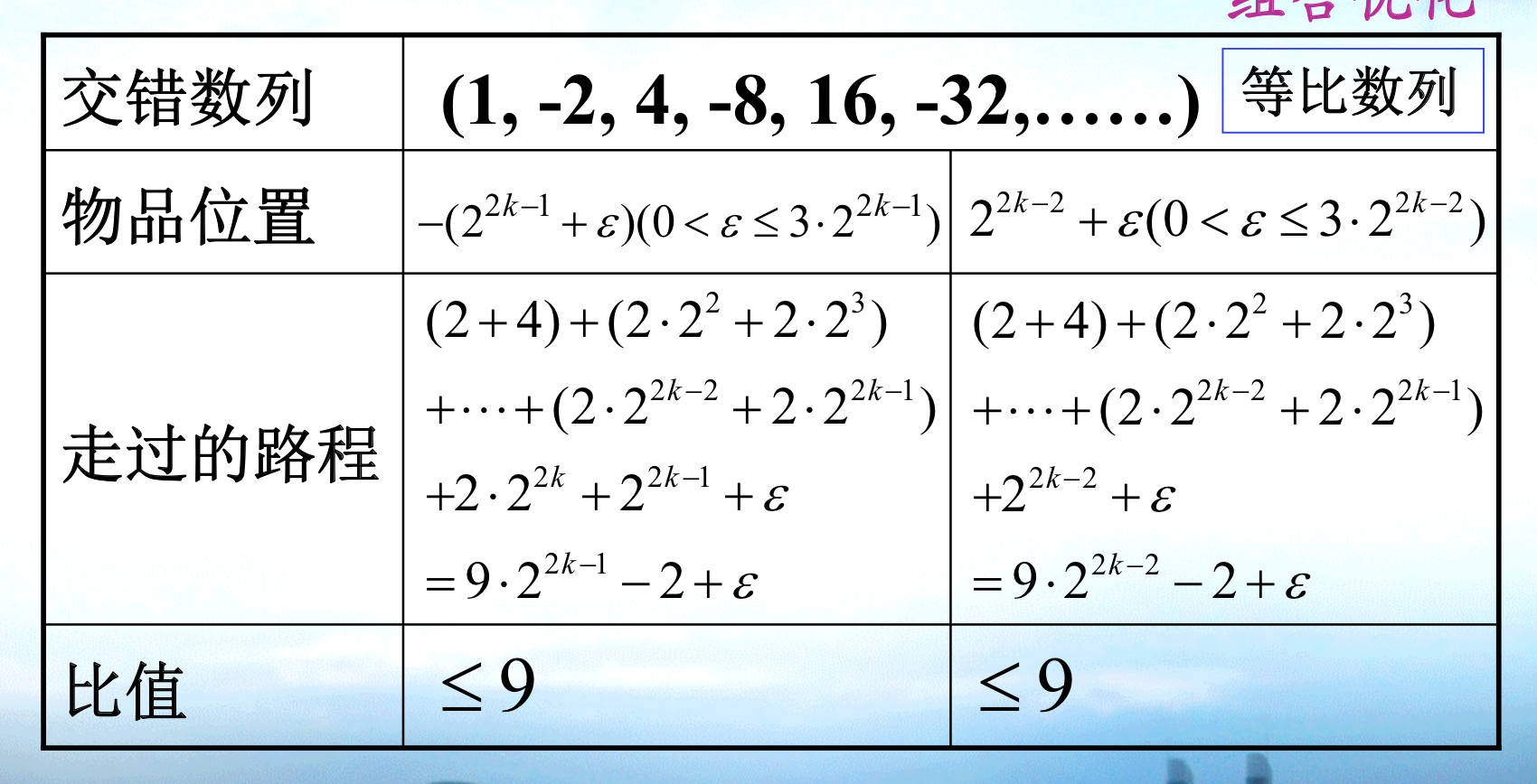
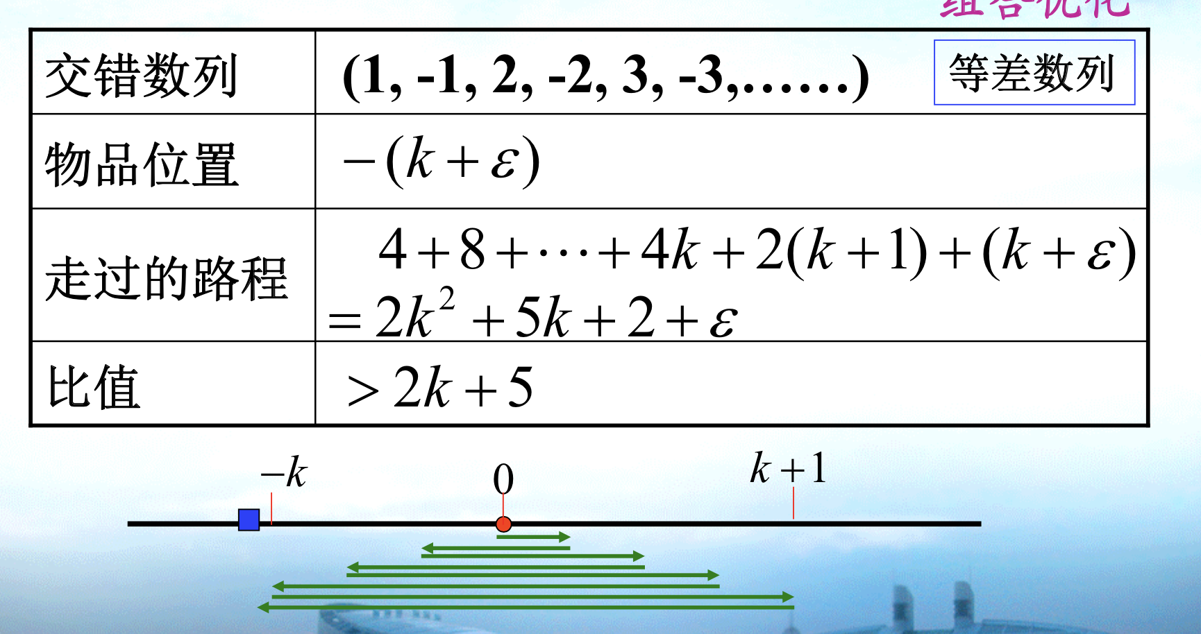
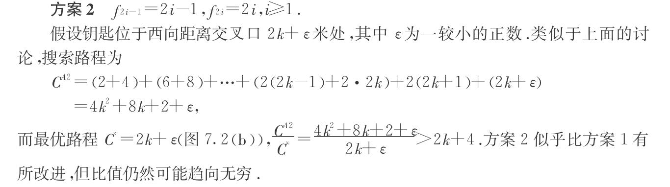
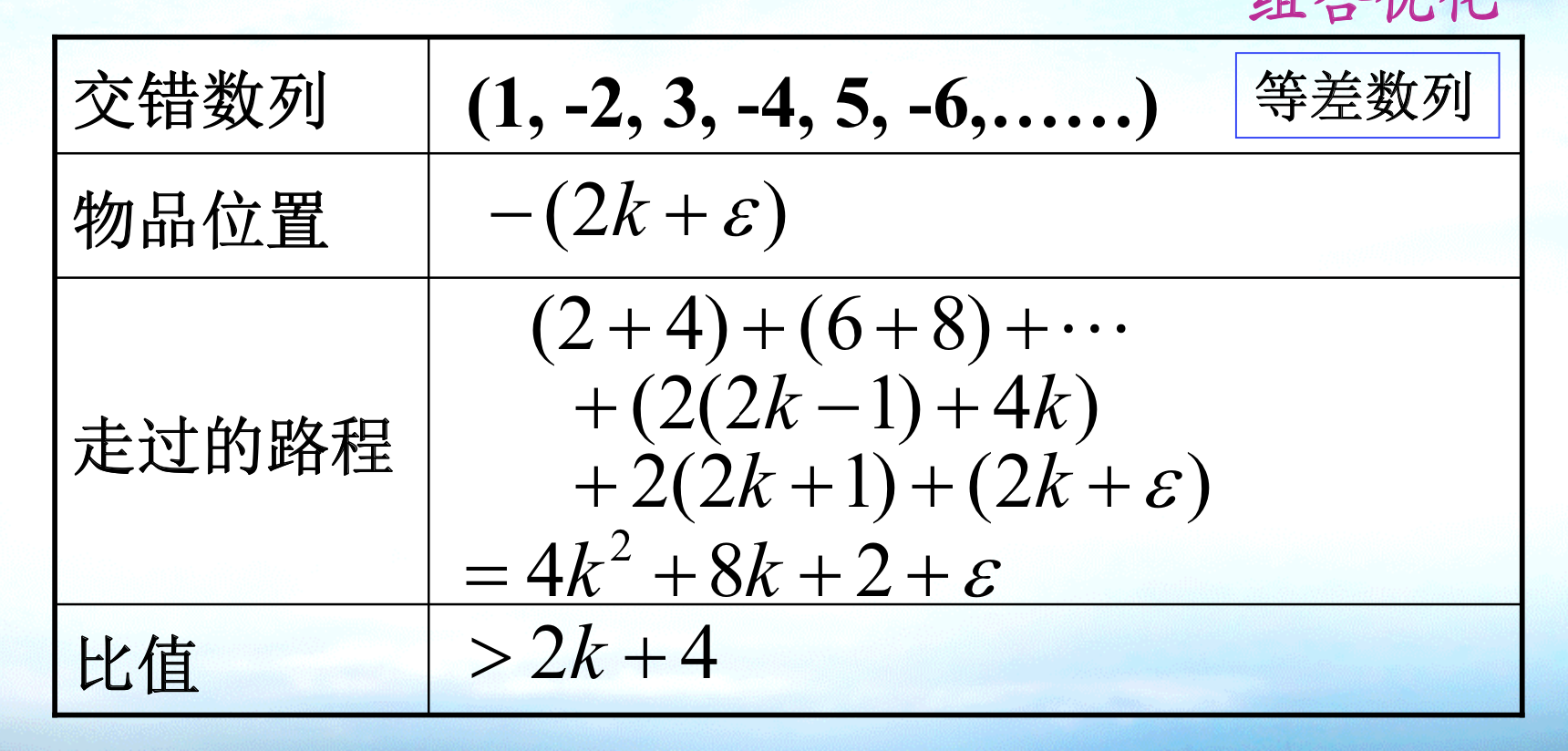
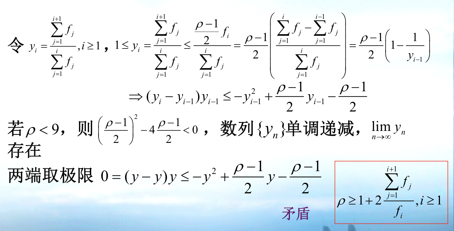
Qua: ratio \(\geq\) 9
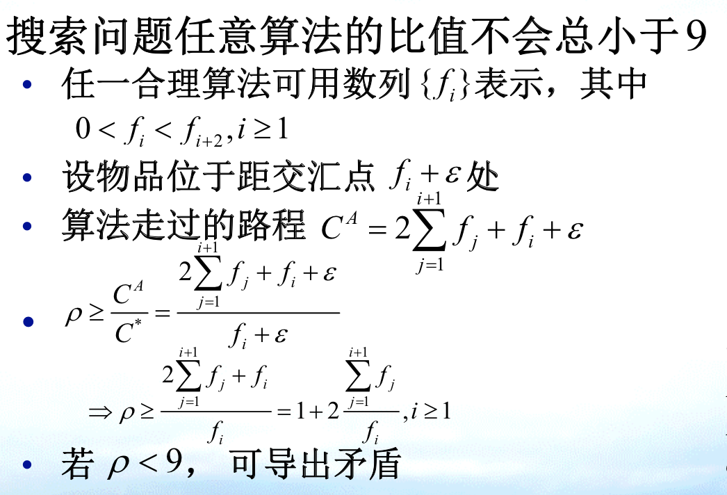
Proof: By construction & contradiction
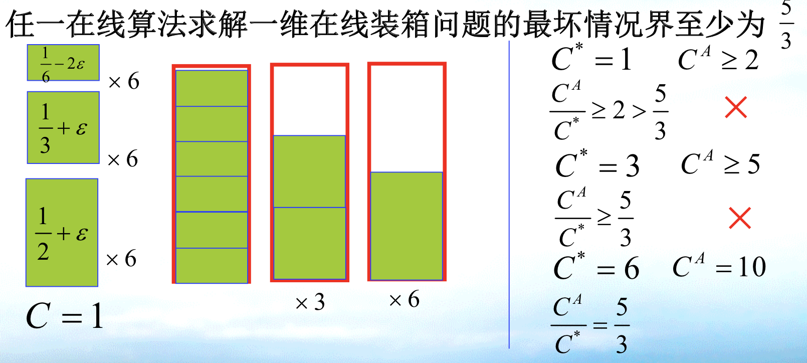
1.18. online bin-packing
Def:
Qua: ratio $$ 5/3
Note: note that we first give 6 1/6 -.., and it'll have to fit in 1. then give 6 1/3, it 'll have to fit in 4. then give 6 1/2, the optimal is 10, we get 5/3. 1)The whole process is about making local greedy optimal worse: 1/6 can be used in optimality but it is used to suffice local optimal. 2)The result is that we make ratio worse: First we get 1/1 => 4/3 => 10/6.
1.19. online scheduling
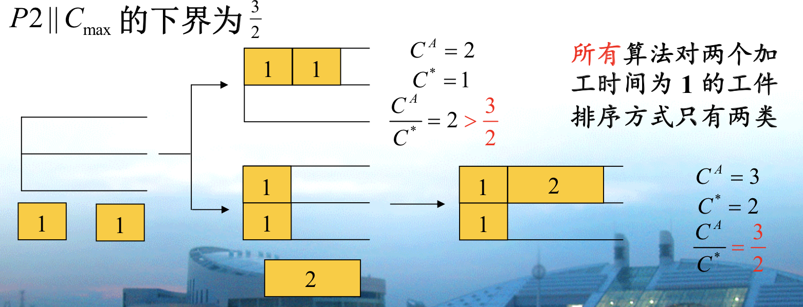
Def: P2||Cmax
Qua: ratio \(\geq\) 3/2
Note: the proof follows the same routine, since 1 can be used in 1 1 / 2, so we have to make it in local optimal solution and make it worse in global optimal solution.
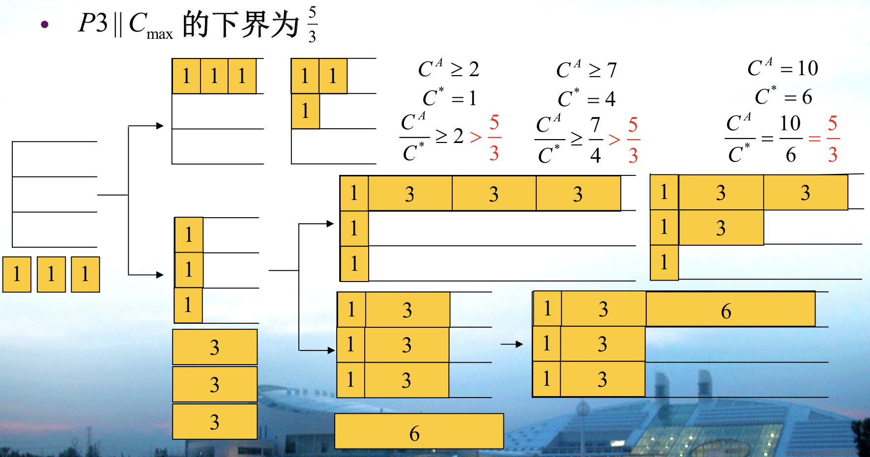
Def: P3 ||Cmax
Qua: ratio \(\geq\) 5/3
2. graph problems
2.1. shortest path
Def: given
Algorithm: 3 classic basic algorithms

2.1.1. dp: Dijkstra
Usage: single source + positive
Def: Dij
1) choose a point with the smallest dis
2) choose the nearest neighbor ( smallest cj)
3) update all point cj
4) set the point as updated()
Note: actually a top-down implementation of bfs, using the feature of principle of optimality, 感觉像是DP算法的进一步优化版本,DP算法尽管有重叠子问题可以消除,但是dij算法还去掉了一些重叠子问题减少计算量(比如在第二个点固定的过程中就只考虑了第一个点的update,其他点都去掉了)
Note: we can generalize the DP algorithm by fixing node by node.
Proof: proof is easy, but note the proof involves in trimming those larger than local smallest, this can not be used in longest path. You can see that the trimming actually trimmed other edges from updating other than the 'fixed' set. The conditions are \(c_ {ij} > 0\). However in longest path, if and only if pj is non-increasing, or \(c_{ij} <0\), this algorithm can be used. \[ p_j = min(p_{smaller set}+cij) \\ p_j \text{ is non-decreasing} \]
Complexity: \(O(e·logv)\): 在核心代码部分,最复杂的是 while 循环和 for 循环嵌套的部分,while 循环最多循环 v 次(v 为顶点个数),for 循环执行次数与边的数目有关,假设顶点数 v 的最大边数是 e。
for 循环中往优先队列中添加删除数据的复杂度为
O(log v)。复杂度 = v个extractmin;E个decreasekey
- 数组 = O(V * V + E * 1) = O(V*V + E)
- 二叉堆 = O(V * lgv + E * lgv) = O((V+E)lgv)
斐波那契堆 = O(Vlgv + E 1) = O(Vlgv + E)
Qua: note that shortest path satisfy DP \[ r_i = \min \limits_{j \in N(i)} (P _{ij} + rj) \]
- Proof: 1) when u->w->v and p'(u->w) is a shorter path than u->w, if p' have no overlap with w->v ,we simply replace u->w with p'
2) when u->w have overlap with w->v, we replace with u->x & x->v where x is the overlapping point.
- Note: that longest path can't prove by this procedure since u->x & x-> v is shorter not longer.
2.1.2. dp: Floyd
Usage: Floyd, all source, negative
D[i][j][k] means the the smallest distance between i and j considering only [1:k] nodes in bewteenDef: Floyd
1) go from k = 1 -> n
2) update i & j (at kth level )
Proof: when k = m, you can prove that with m nodes in between, the update is valid. If not, after the update, there exists some node gg $$ [1, m], and \(i^*\to gg + gg \to j^* < i \to gg + gg \to j\) , so that either i->gg or gg->n is not the smallest path.
- Note: intuition is if left is shortest path and right is shortest path then the middle is shortest path. we can generalize the DP algorithm by fixing layer by layer such that the update path only concerns k nodes.
Complexity: $O(n^3) $
2.1.3. dp: Bellman-Ford
Usage: single source + negative circle

Def:
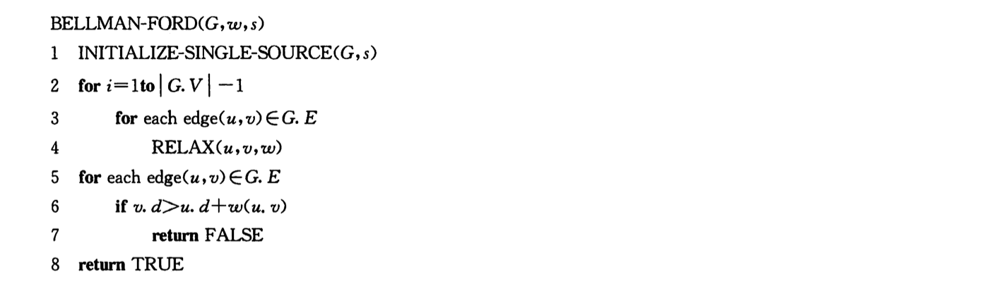
- Note: every edge relaxation V-1 times, if can still relax => negative circle, if not return v.d
Proof: every round at least 1 edge is fixed, then we need at most n-1 round to fix everyone.
Complexity:

2.1.4. dp: DAG
Usage: DAG + single source + negative
Def:
2.2. strongly connected components
2.2.1. dfs
Usage: to find SCC
Def:

Theorem:

Note: this theorem means we can draw a graph like this

Theorem:

- Note: this theorem means abe = 4 cd = 3 h = 2 fg =1, high goes to low. which means we revert the graph, and start from high, then all pathes from high to low are cut, then we can find the components.
2.3. minimum spanning tree
Def: eliminate edge
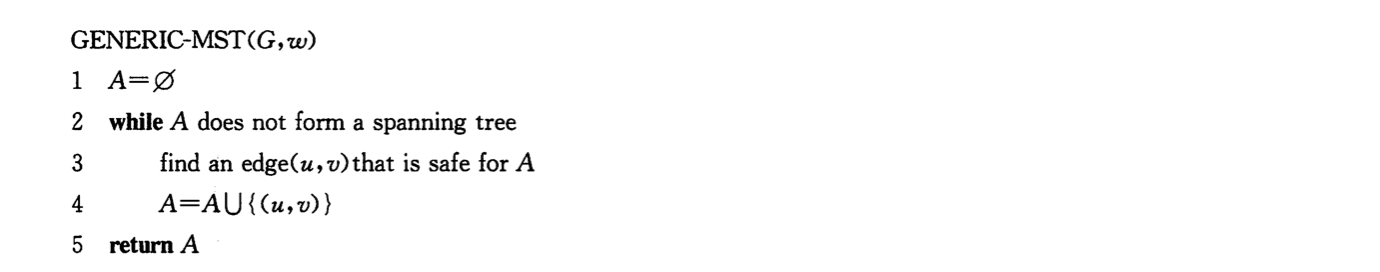
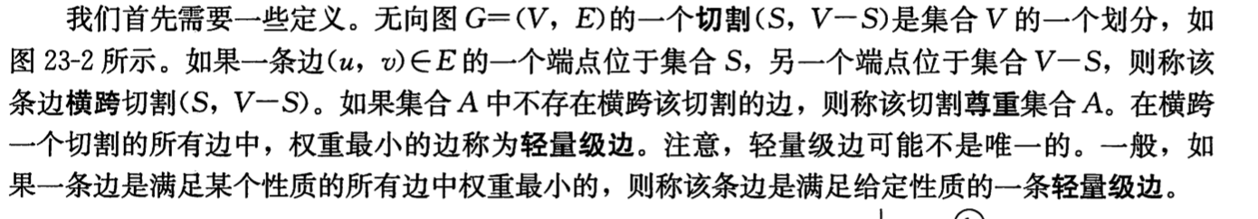
Def: 切割
Theorem: safe edge

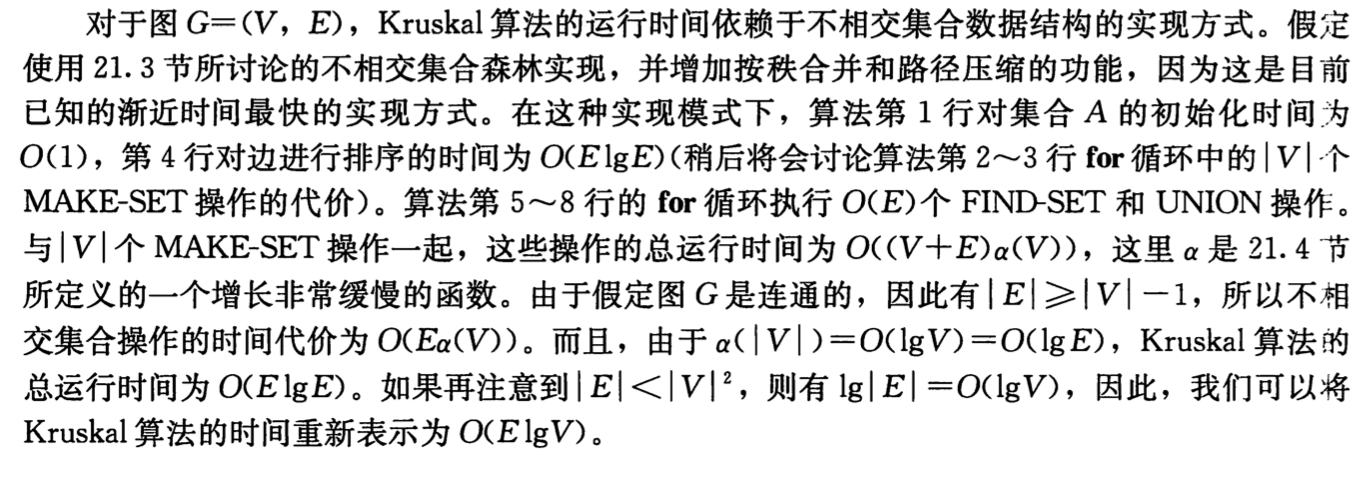
2.3.1. other: Kruskal
Def: Kruskal
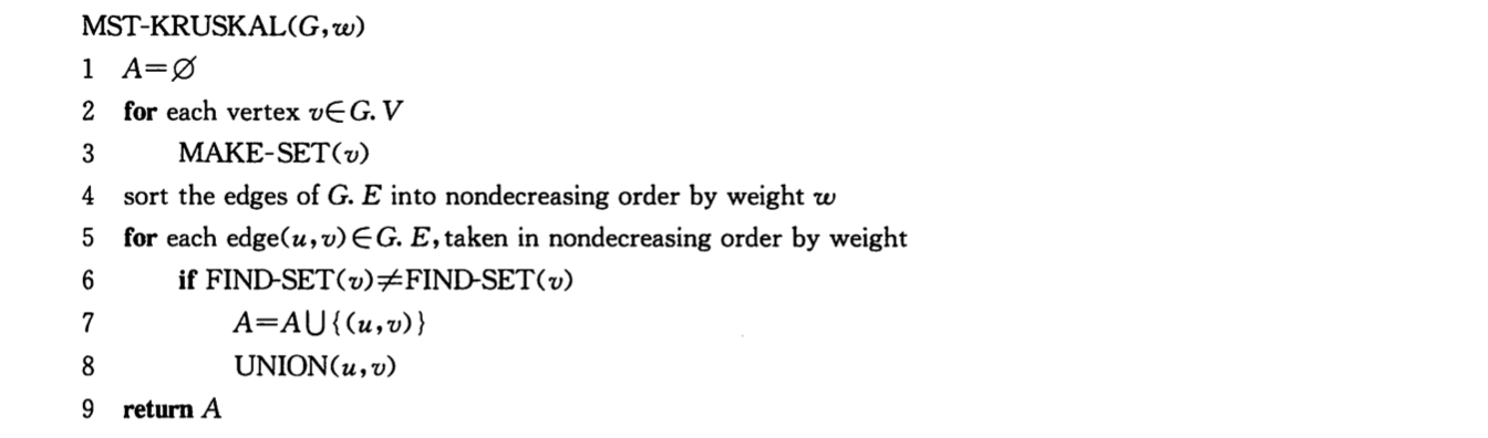
Note: add edges with no circle
Complexity:
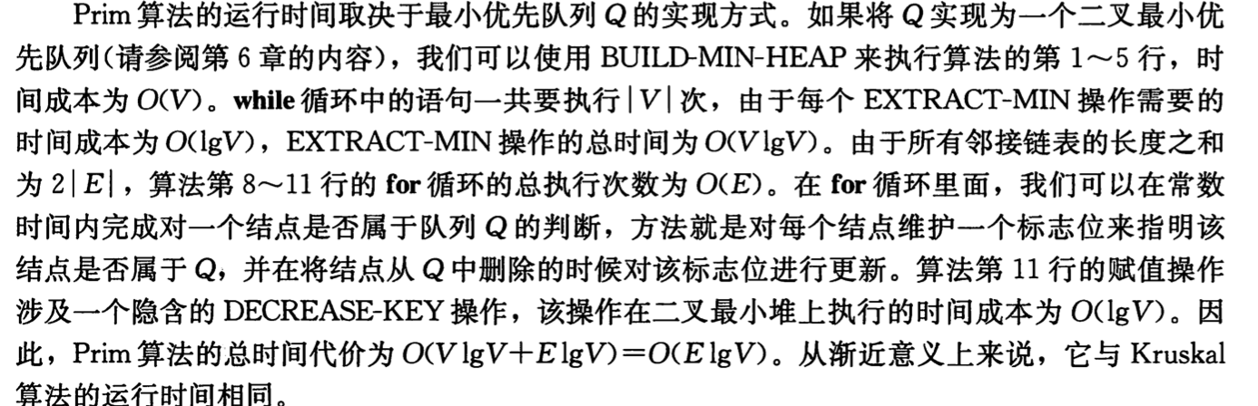
2.3.2. other: prim
Def: prim
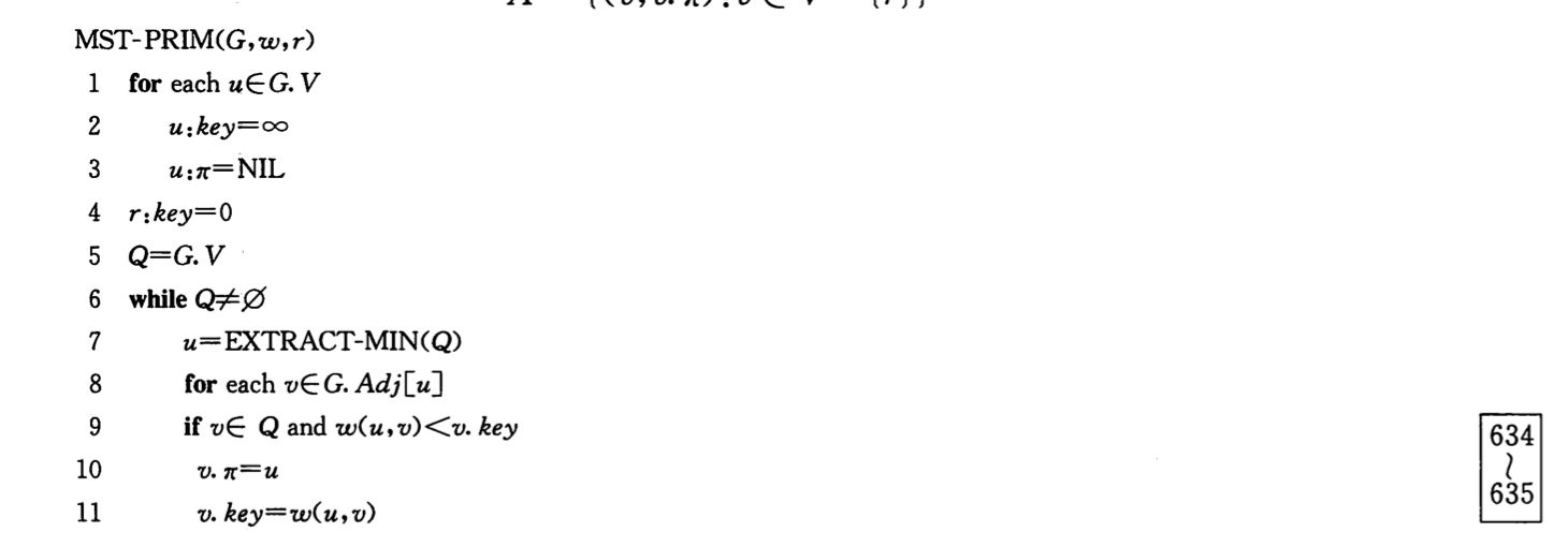
Note: add node with min distant with current set.
Complexity :
2.4. max flow
Def: flow network
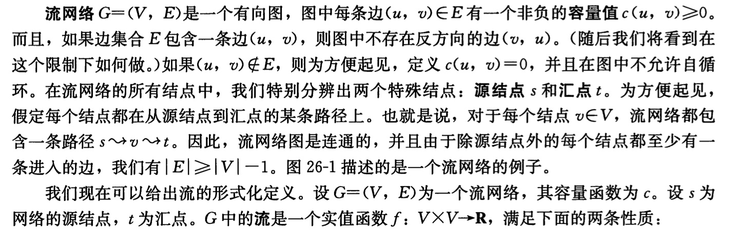
Def: max flow problem
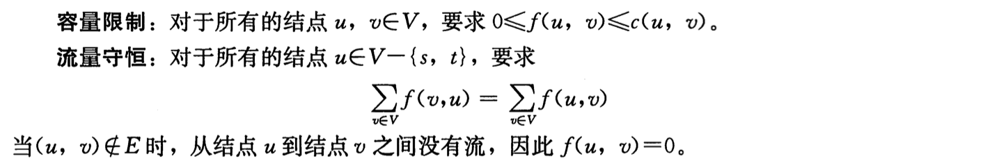
Def: flow & residual network
Note: 同向相减,反向用总-同向
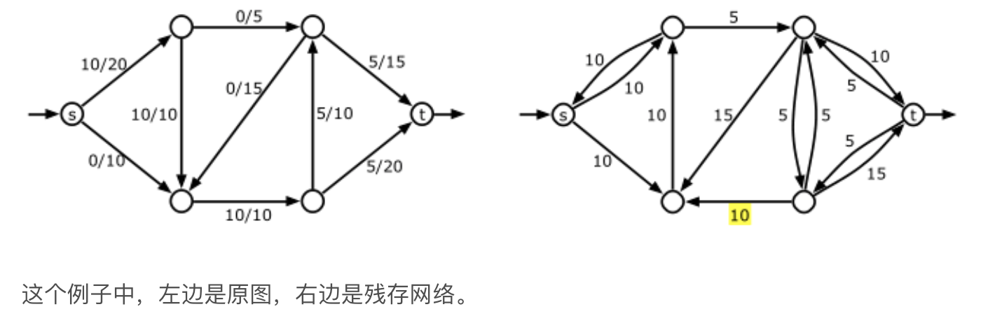
Def: segment path
Def: augmentation
Theorem: => that f+f' is a flow

Def: cut
Note:
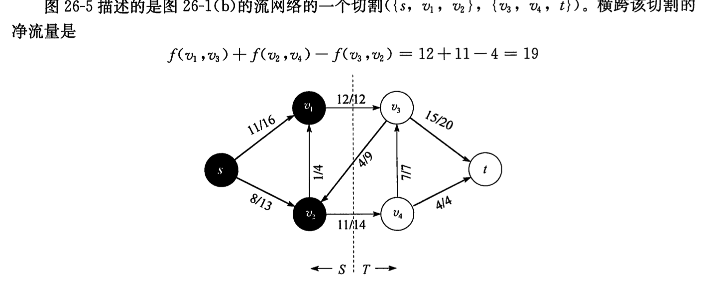
Theorem: flow & cut

Theorem: max flow = min


Proof:
Note: 给定 flow value = 任意 cut 流量 <= 任意 cut 容量。所以如果有flow value达到最小cut容量,它必然是最大的。
2.4.1. other: Ford-Fulkerson
Def: Ford-Fulkerson
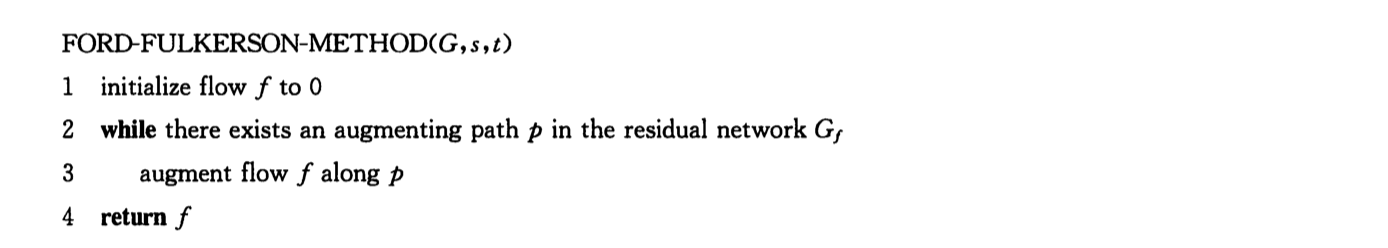
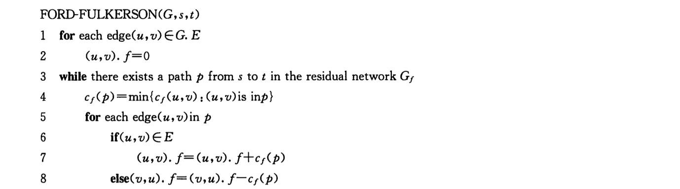
- Note: find possible path & add it to the flow .
Complexity :
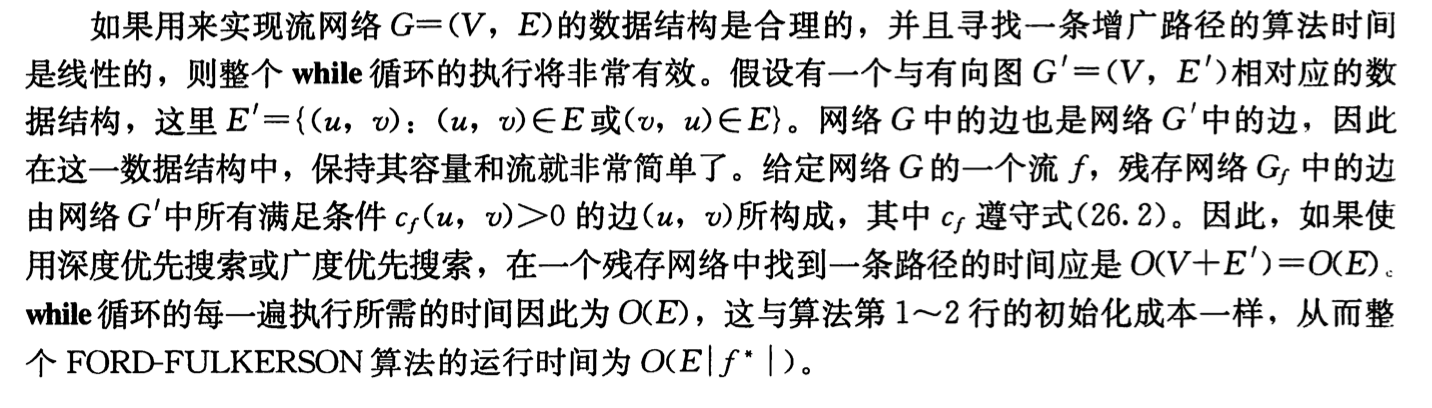
2.4.2. bfs: Edmonds-Karp
Usage: improved Ford

Complexity: \(O(VE^2)\)
2.5. metric TSP
Def: metric tsp
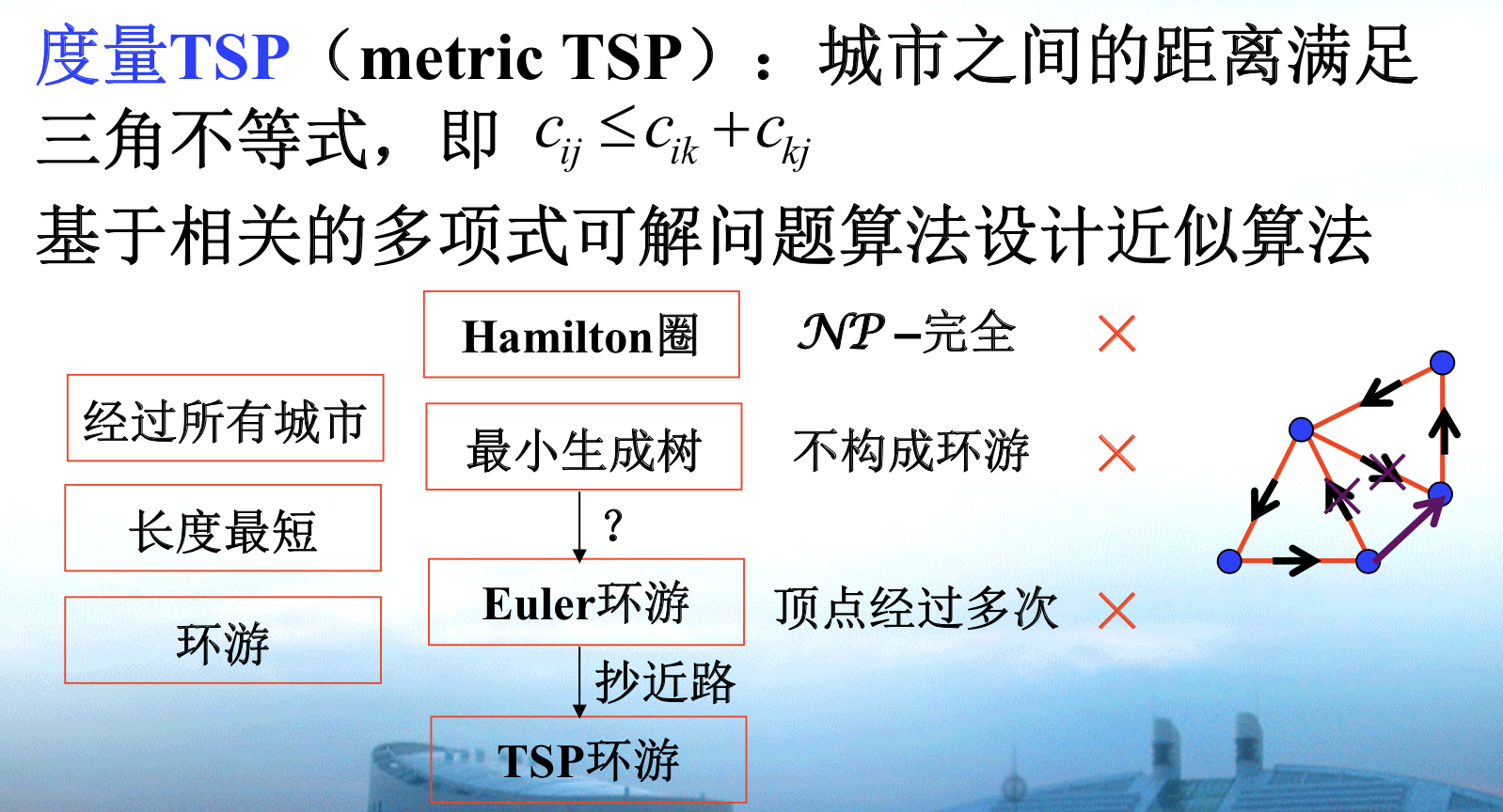
2.5.1. other: Kruskal
Algorithm: weighed smallest spanning tree method
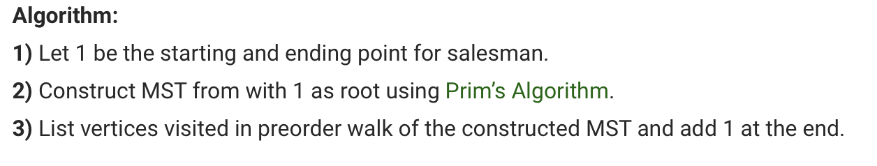
Qua: => appximate ratio = 2

Proof: we need to prove that 2xtree will always suffice to make it larger than Cdm. By that I mean the edges will always be enough to eliminate edges in Cdm. since the degree of nodes can't be three, we proved the point.
Note: Lt act like a LB for C*.
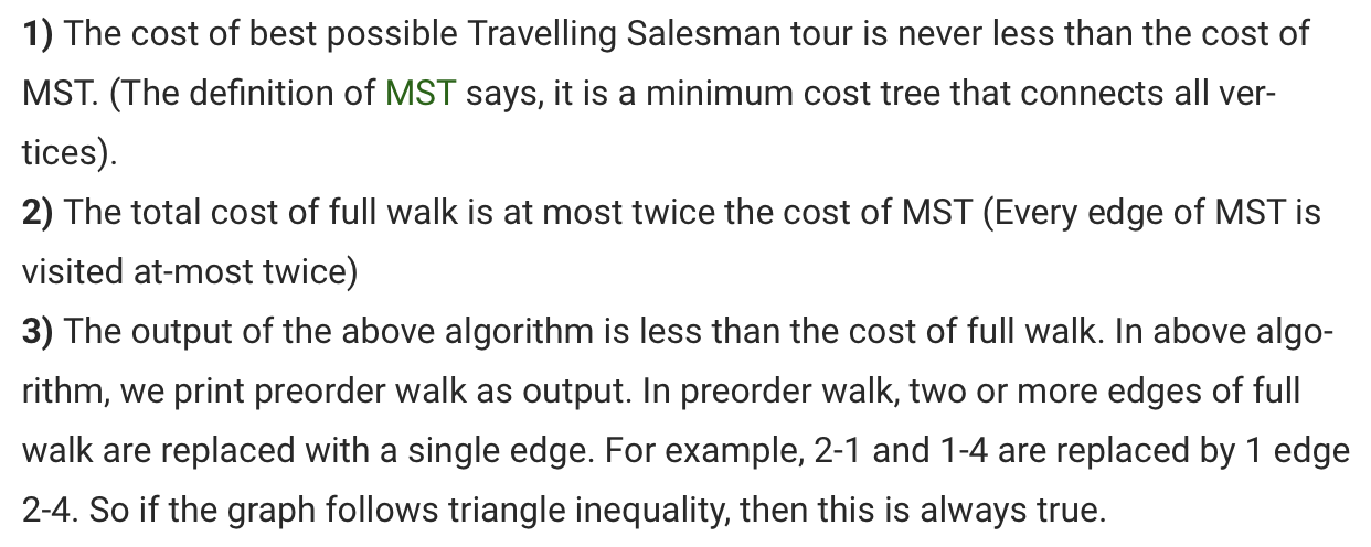
Qua: => the best approximate ratio = 2
Proof: given an example of worst ratio
2.5.2. other: christofides(spanningtree+minmatch)
Algorithm: christofides
Usage: note that euler tour can be redundunt on edges as long as you past every edge in the M+T
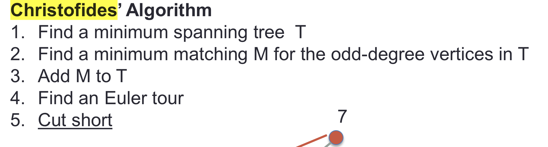
Qua: => ratio \(\leq\) 3/2
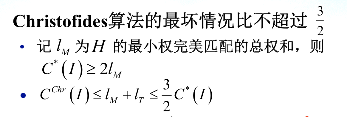
Proof: first we prove that T< C, this is easy since we can erase edge from C and T<C-edge<C. Then we can see that Chr = M+T - Euler overlap < M+T < M + C. And C > C - evenpoint >= 2 * M . So M<=C/2, Chr< 3/2 C.
Note: C- evenpoint, and this is the lower bound of C which is very important.
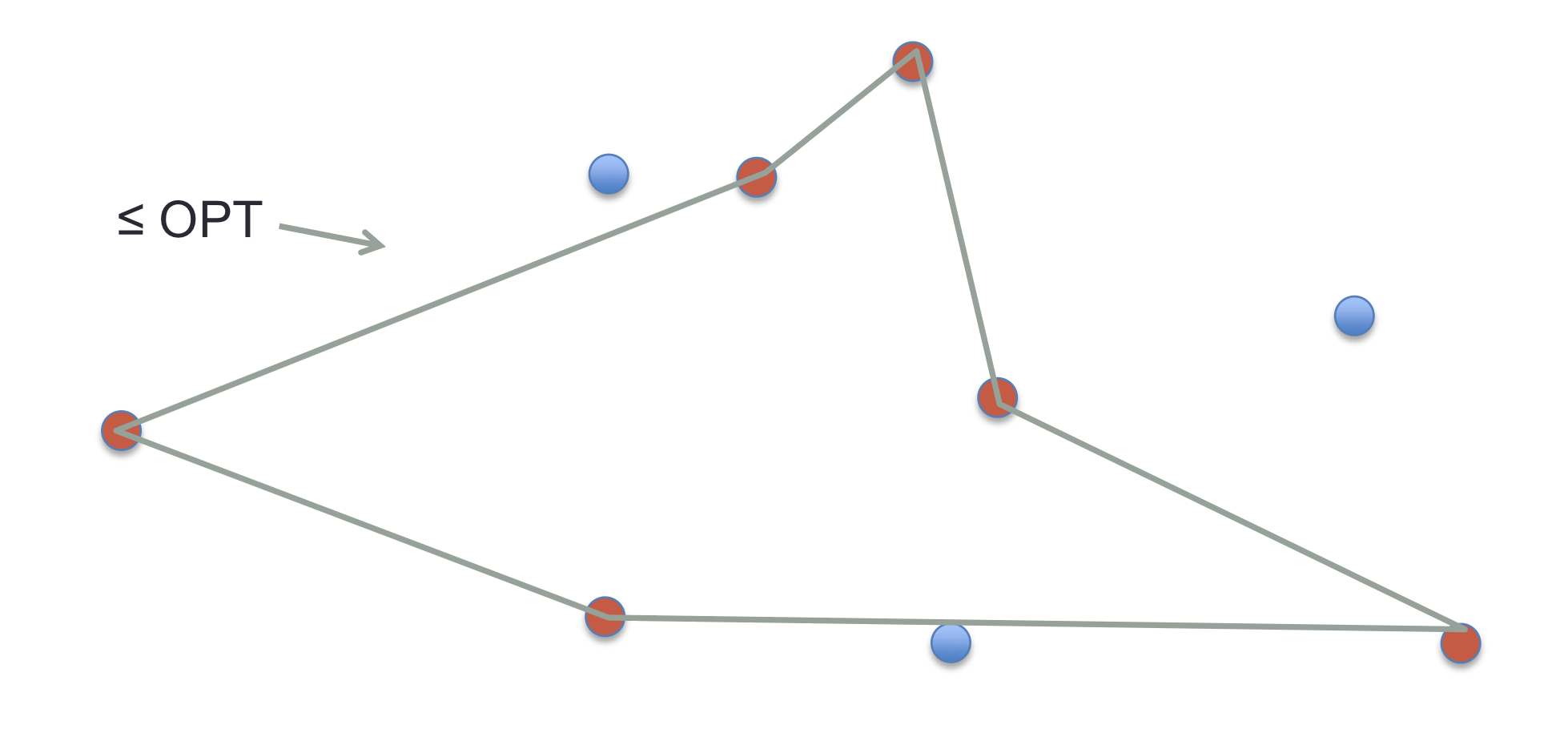
Qua:worst ratio \(\geq 3/2\)
2.6. tsp problem
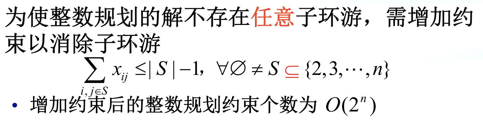
Def: tsp problem (same as assignment ) (this is not the final version)
img Note: sub-tsp have to be mentioned. sub-tsp have to be mentioned, the problem can be separated into several small problems if the constraint is not mentioned.
Qua: first solution
Proof: since the only 2 conditions are: from 1 -> 1 / 1-> 1 + j -> j, we eliminate the second condition.
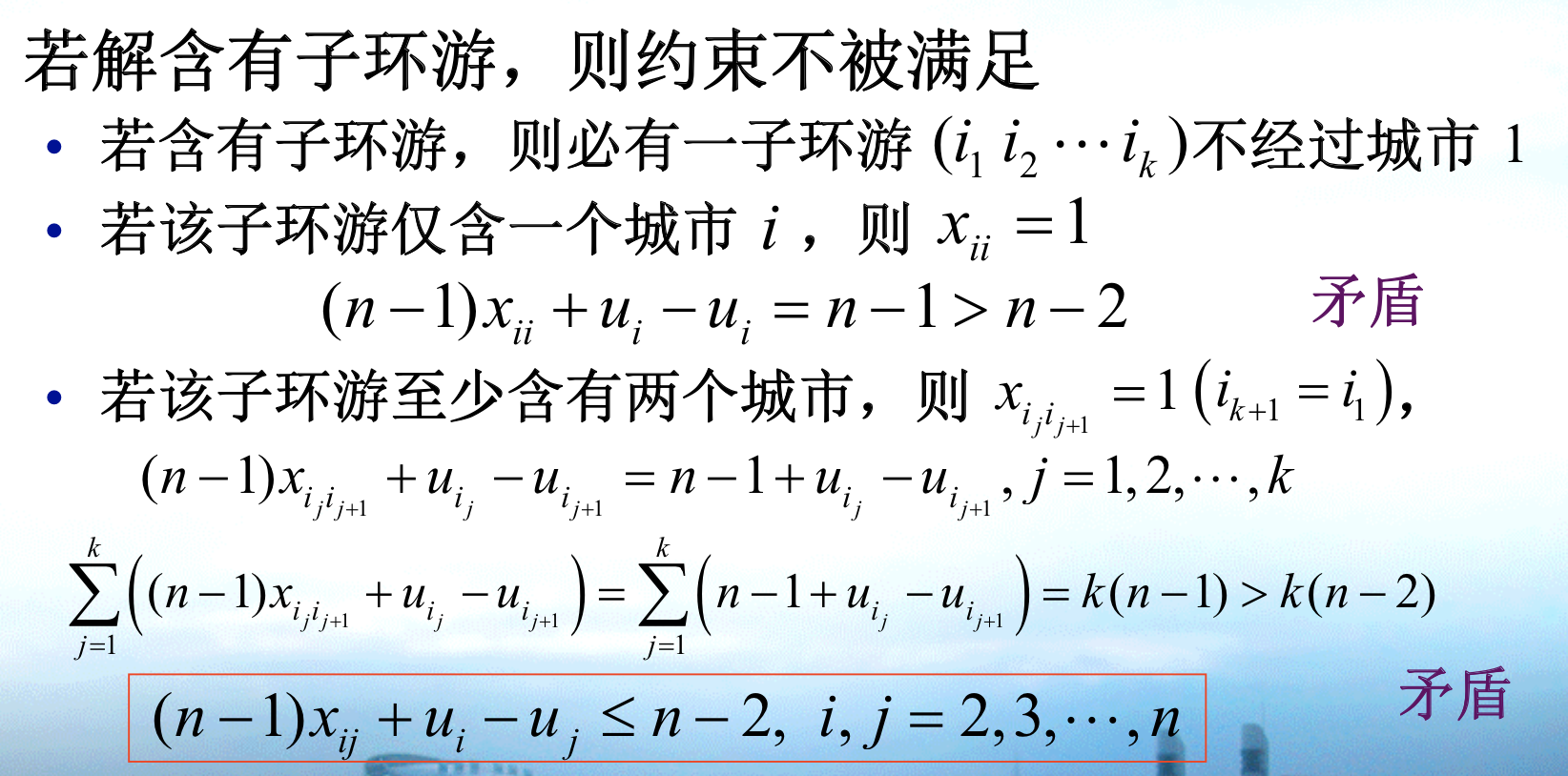
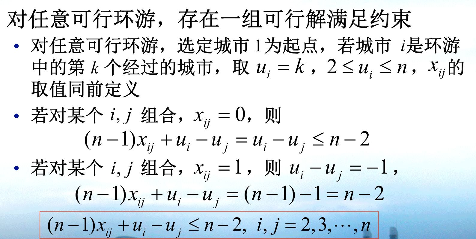
img Qua: second solution

img Proof: note that the given condition makes that every
=>
img <=
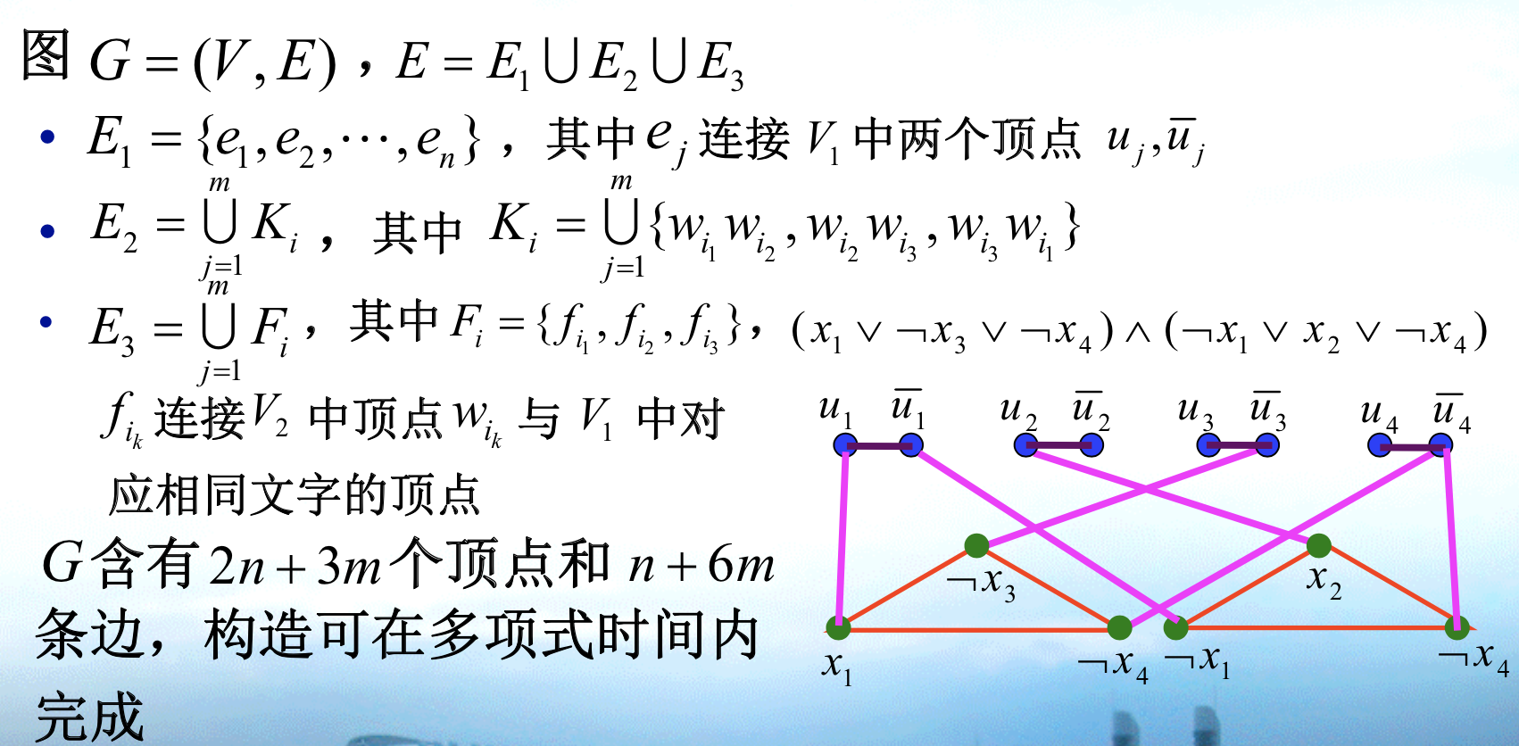
img Qua: NP-C
Qua: no constant - ratio
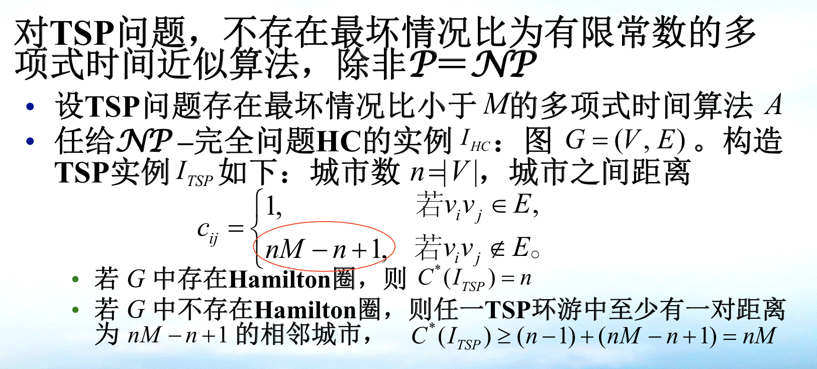
img Proof: using reduction to HC, which is a NPC problem, (gap technique)
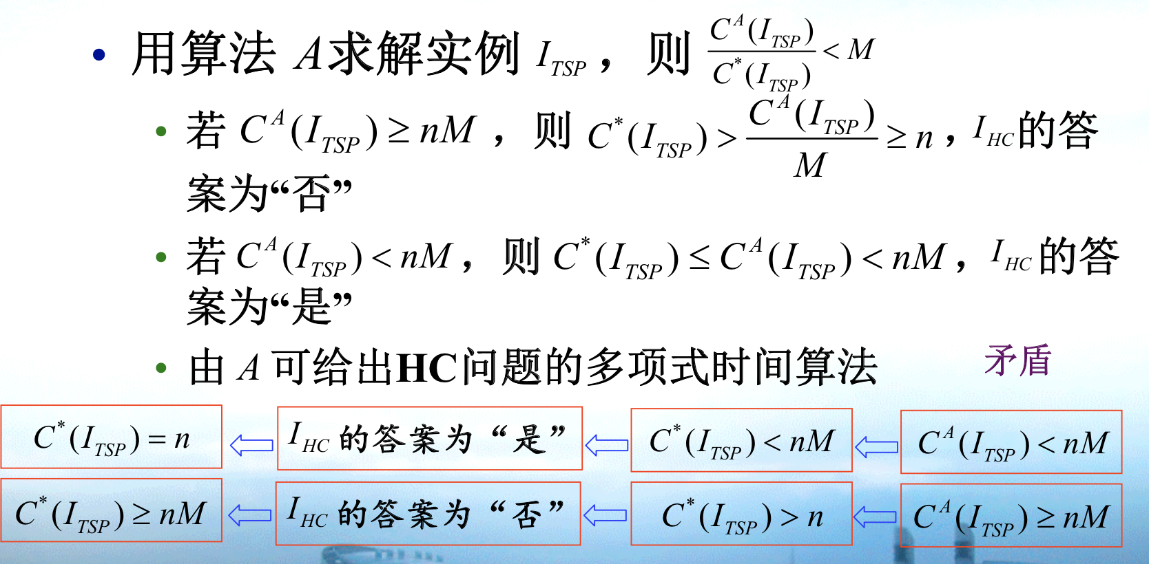
img Qua: no FPTA
2.7. take-out problem (specific shortest path)
Def: a special form of shortest path,

img 
img
2.7.1. dp
Algo: dynamic programming

img 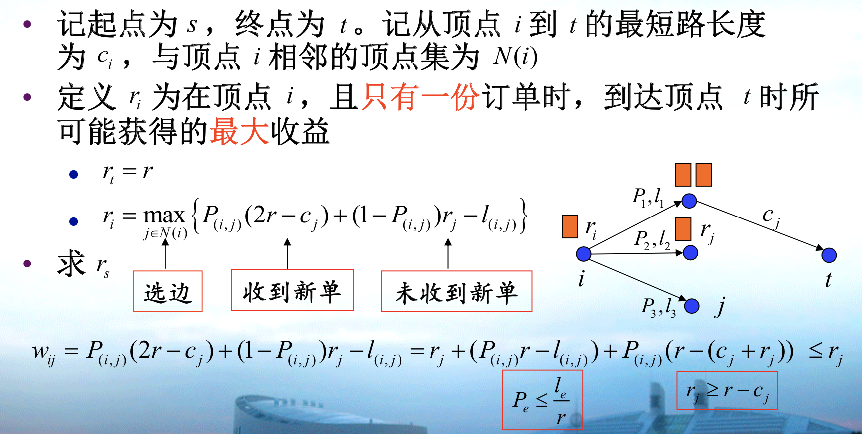
img implementation( here min should be max and wjt = max里面的内容 )
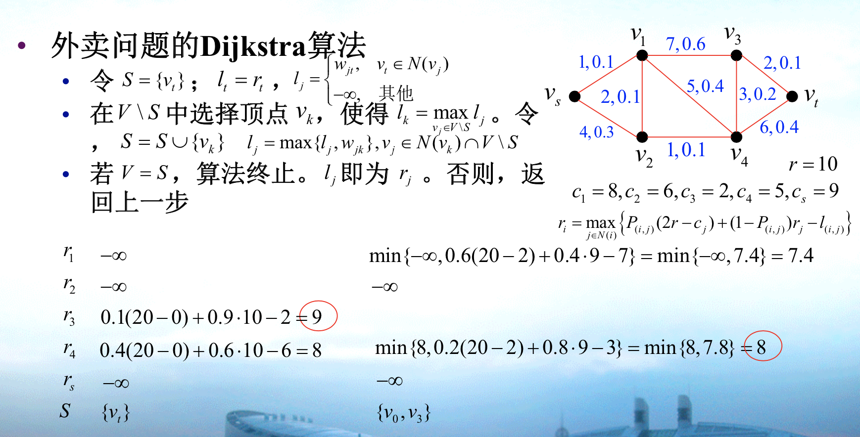
img Note: use special form of Dij algorithm to solve it. You can see that rj is non-increasing/ 直接加两个负号,-ri = min(-ri+l1)变成最短路问题(最短路问题l1验证必须为正)
2.8. minimum matching
Def: minimum matching
Usage: matching 问题简而言之就是找一个边集,使得任意顶点只有一条边。

img
2.9. vertex cover
Def: vertex cover
img 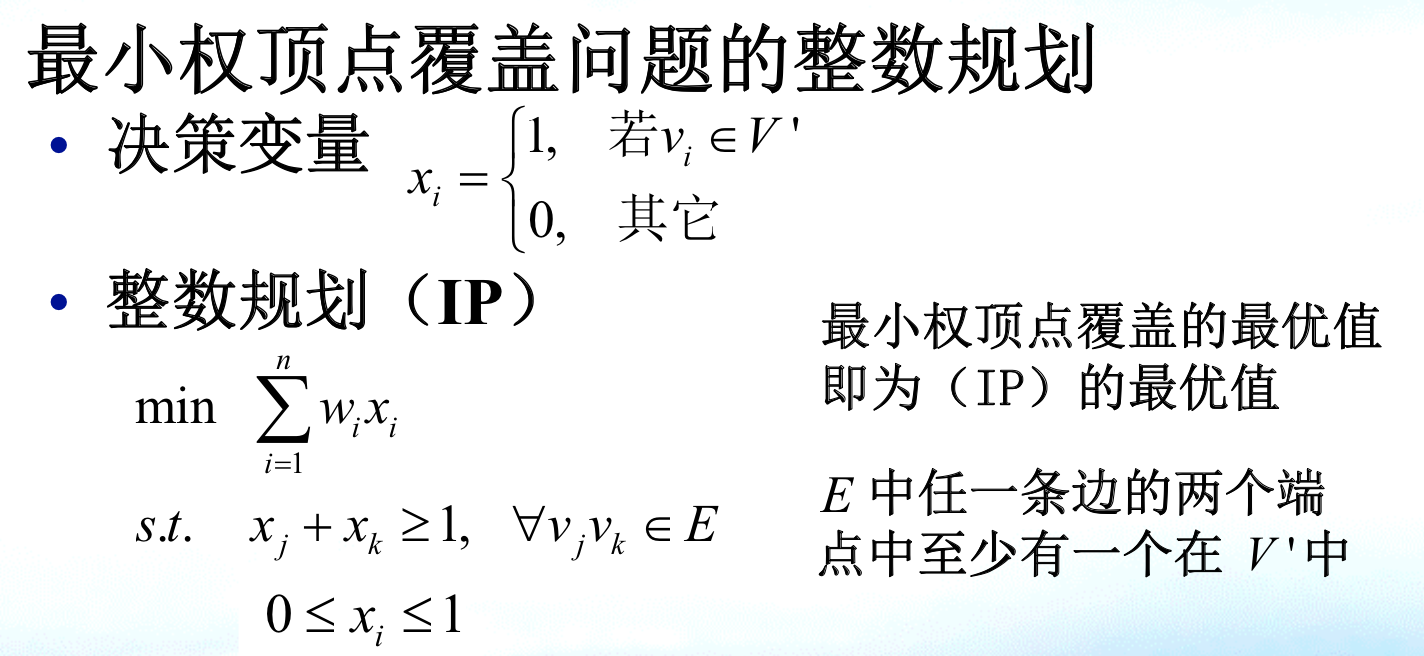
img Qua: NPC
Proof: 3SAT VC
img => 通过给=1的顶点染色,然后给剩下三角形的两个染色,证明是VC
<= 先证明如果是VC上面必须有n个,下面也必须有2m个,又因为条件里有《n+2m,所以=n+2m个,然后就证完了。
2.9.1. linear programming: relaxation algorithm
Algo: relaxation algorithms
Qua: => ratio 2
Proof: LP is natural lower bound.
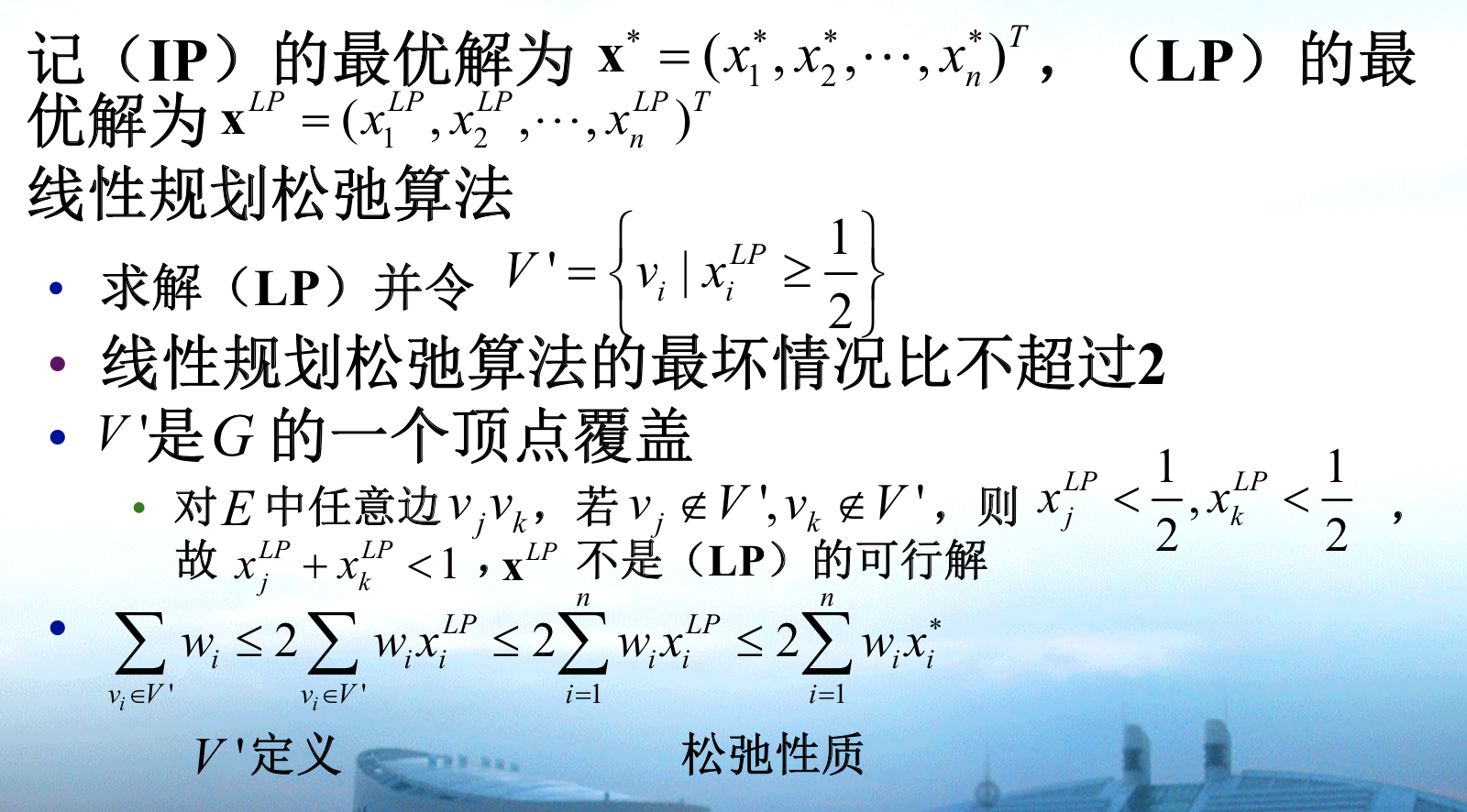
img
2.9.2. random: local search
Algorithm :

Qua: ratio = bad
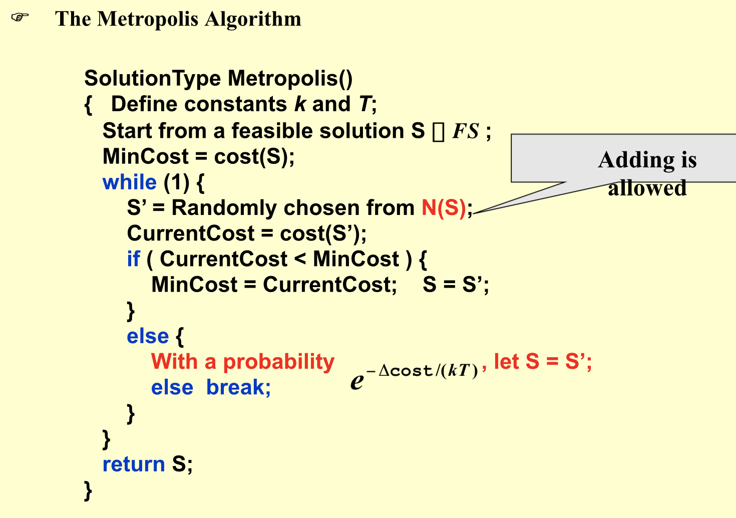
2.9.3. random: metropolis
Algorithm:
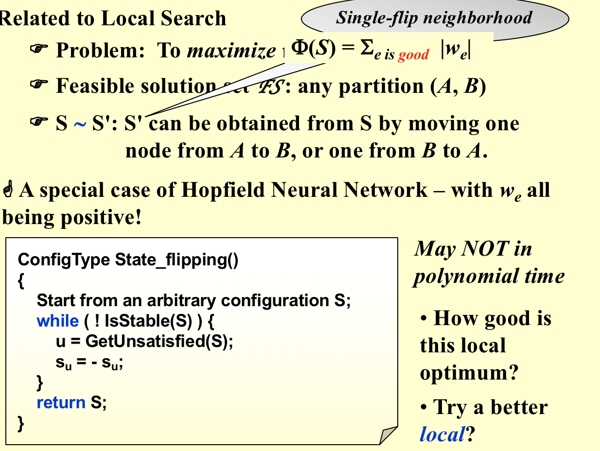
2.10. hopfield network
Def:
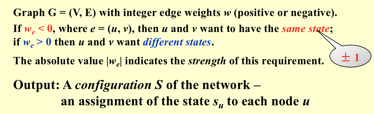
Def:
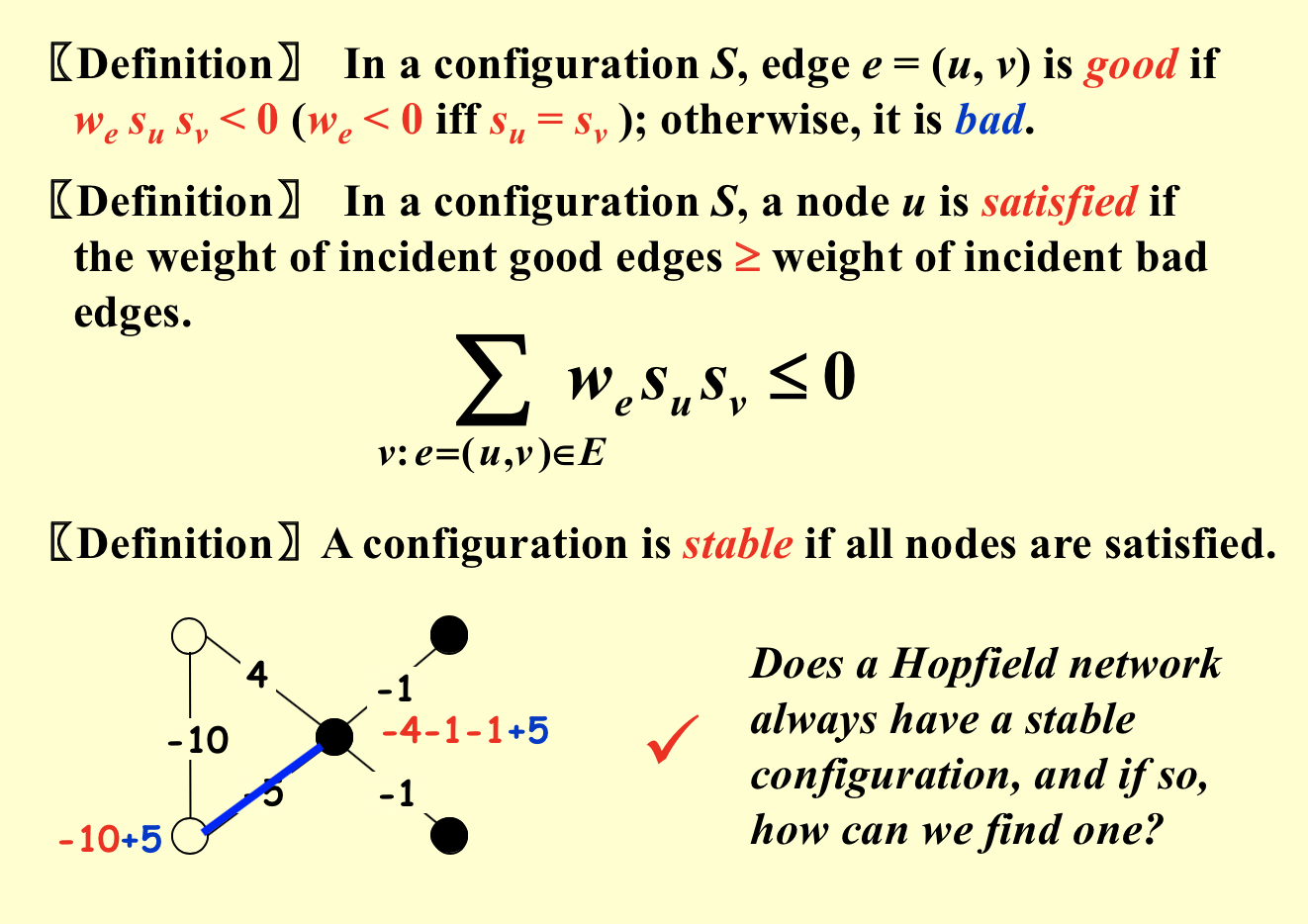
2.10.1. local search
Def:
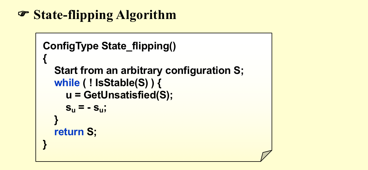
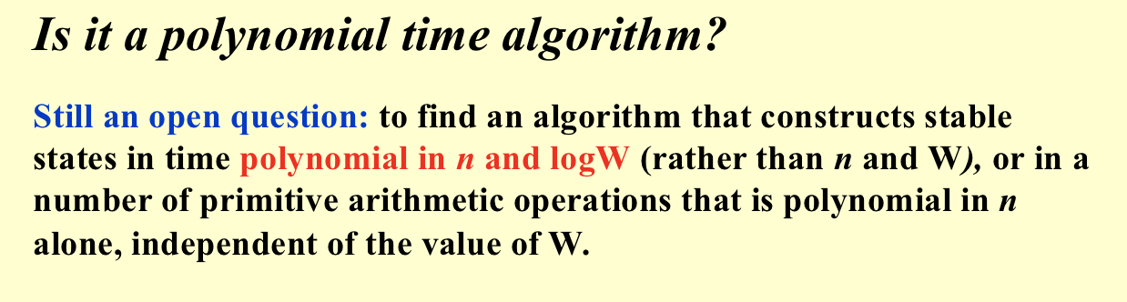
Qua: will terminate
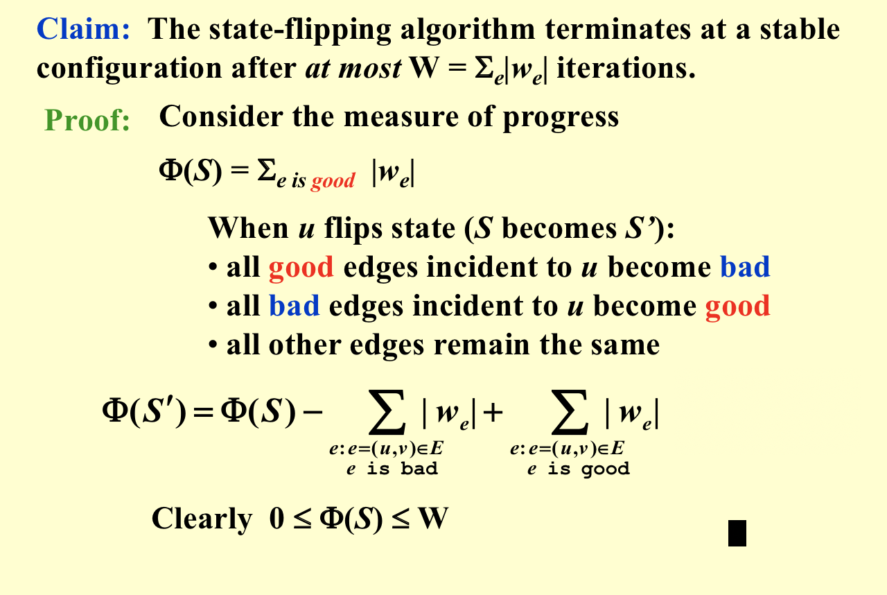
Complexity :
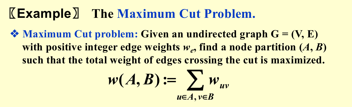
2.11. max cut
Def;
2.11.1. random: local search
Algorithm:
Qua: ratio = 2
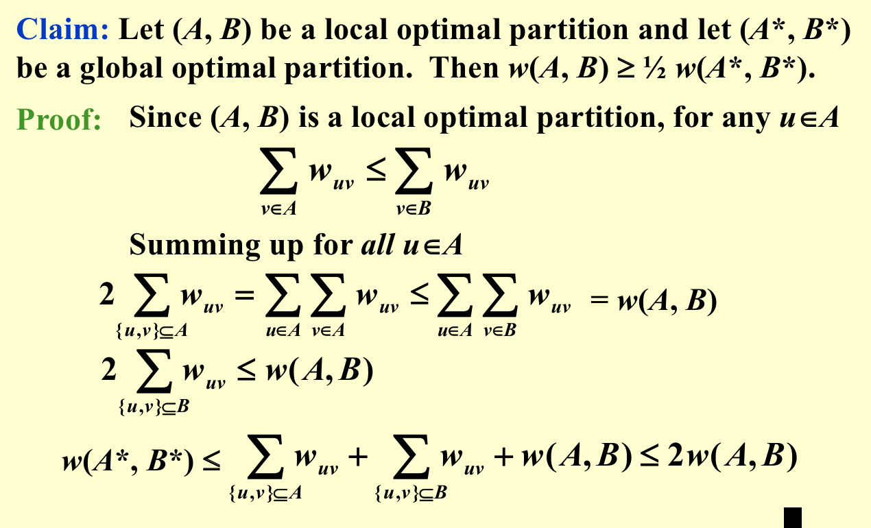
Qua :
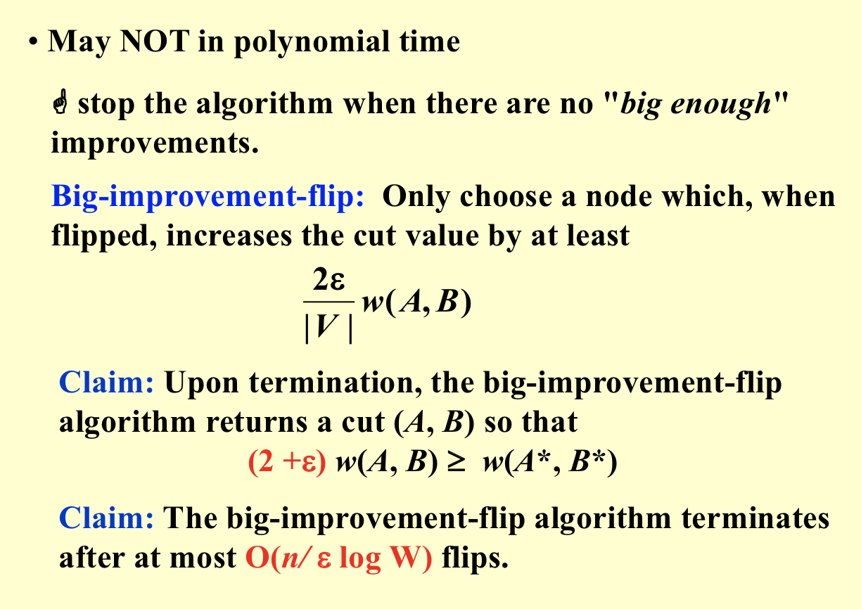
2.11.2. random: local search improvement
Algorithm:
3. strategy problem
- Def: strategy problem anyway, can't be categoried into optimization problem(with a programming structure)
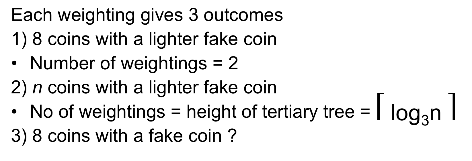
3.1. fake coin weighing
- Def :check out ligher coin
3.1.1. weighing
Def: split into 3 parts, n, n, n-1/n-2.