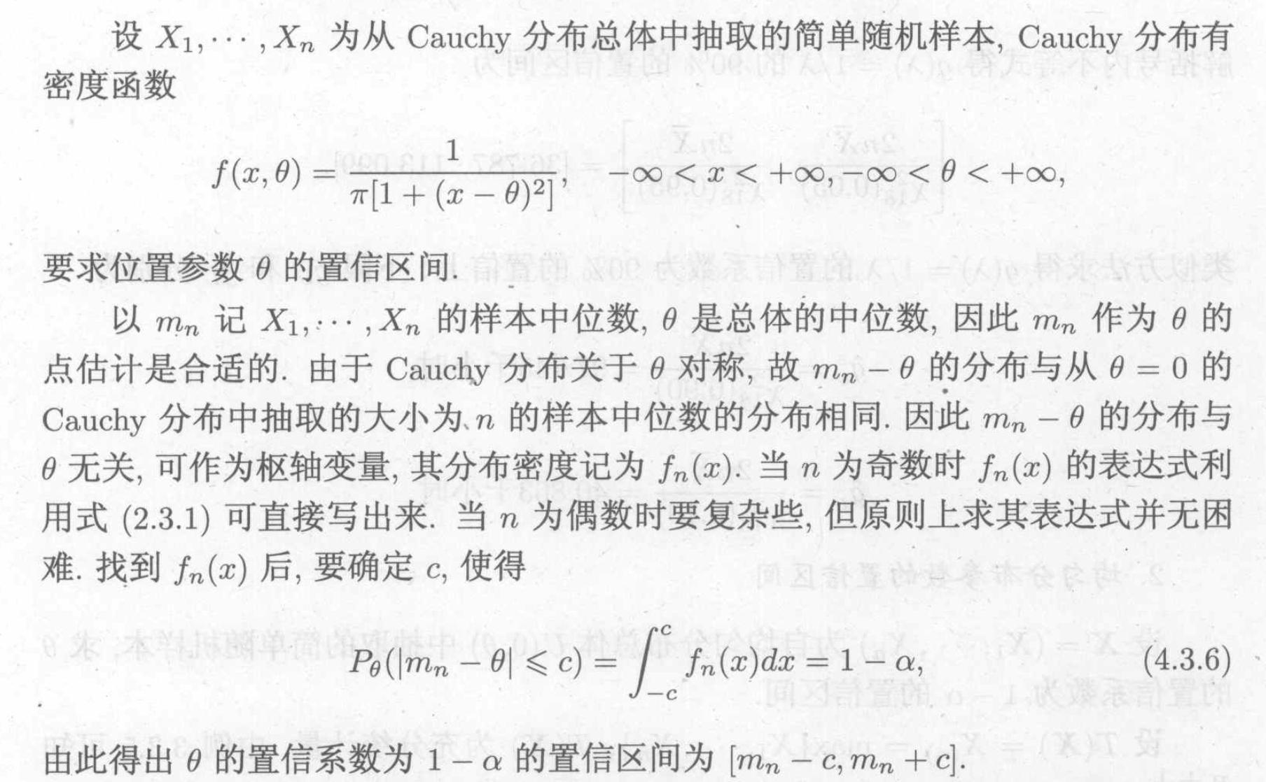
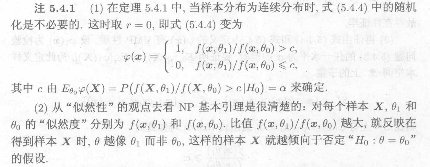
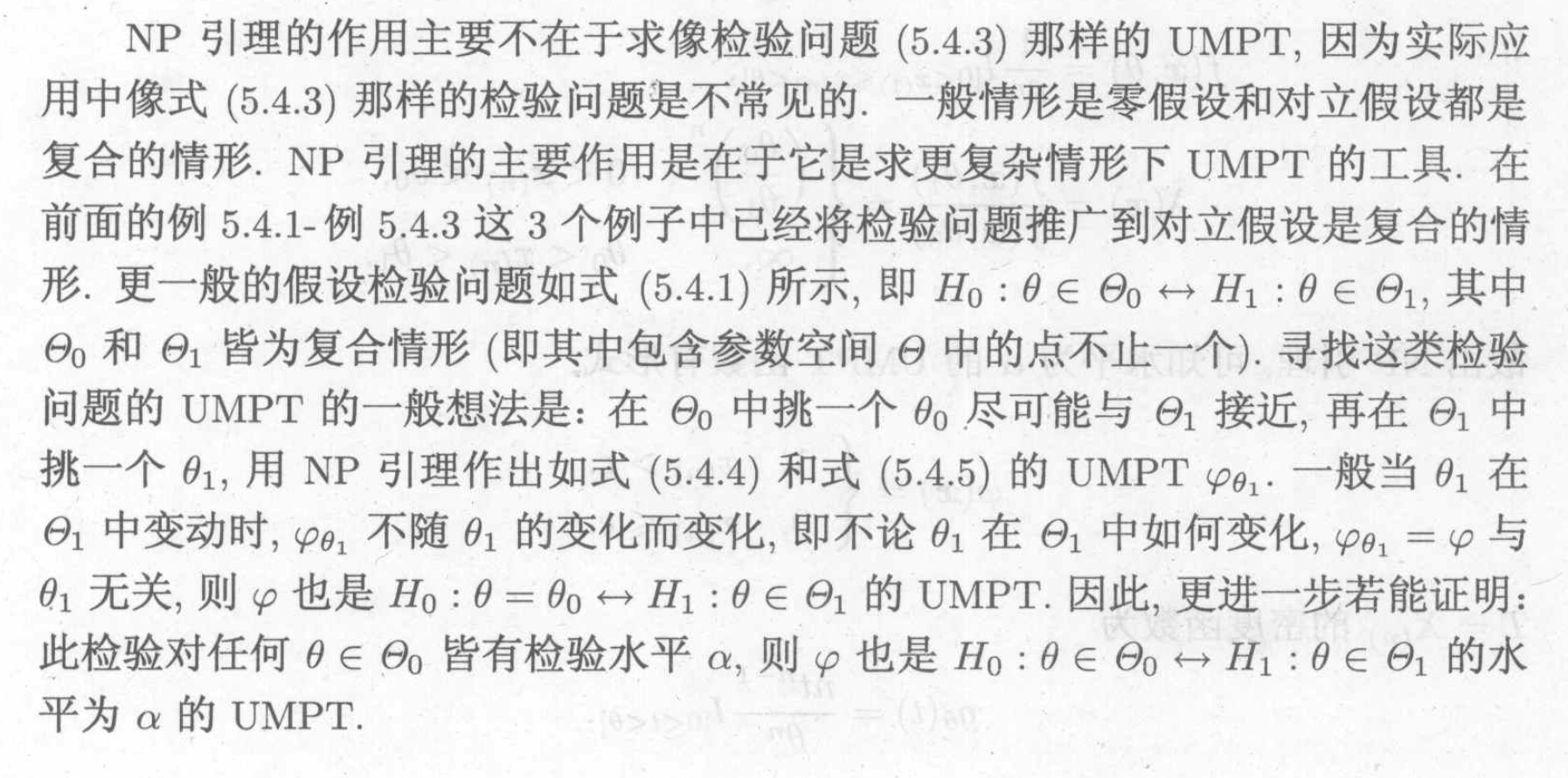
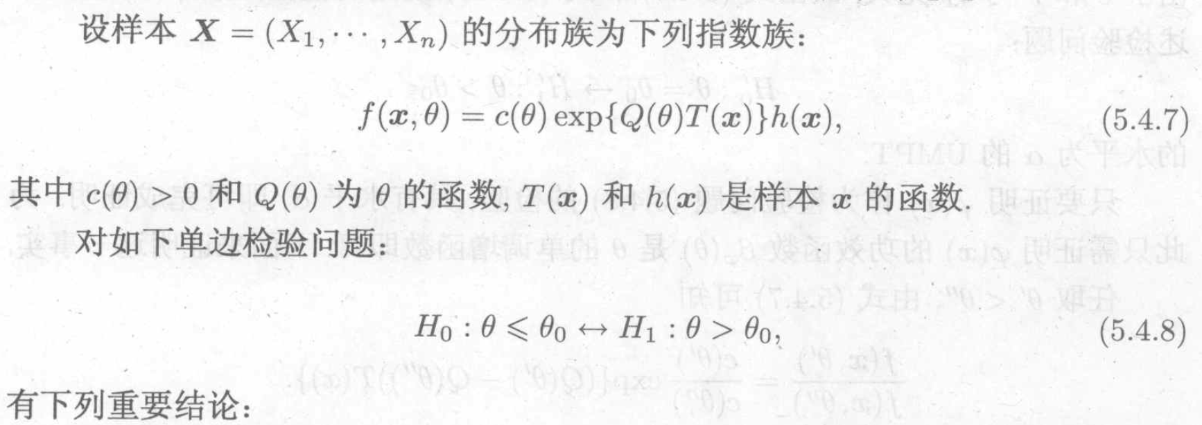
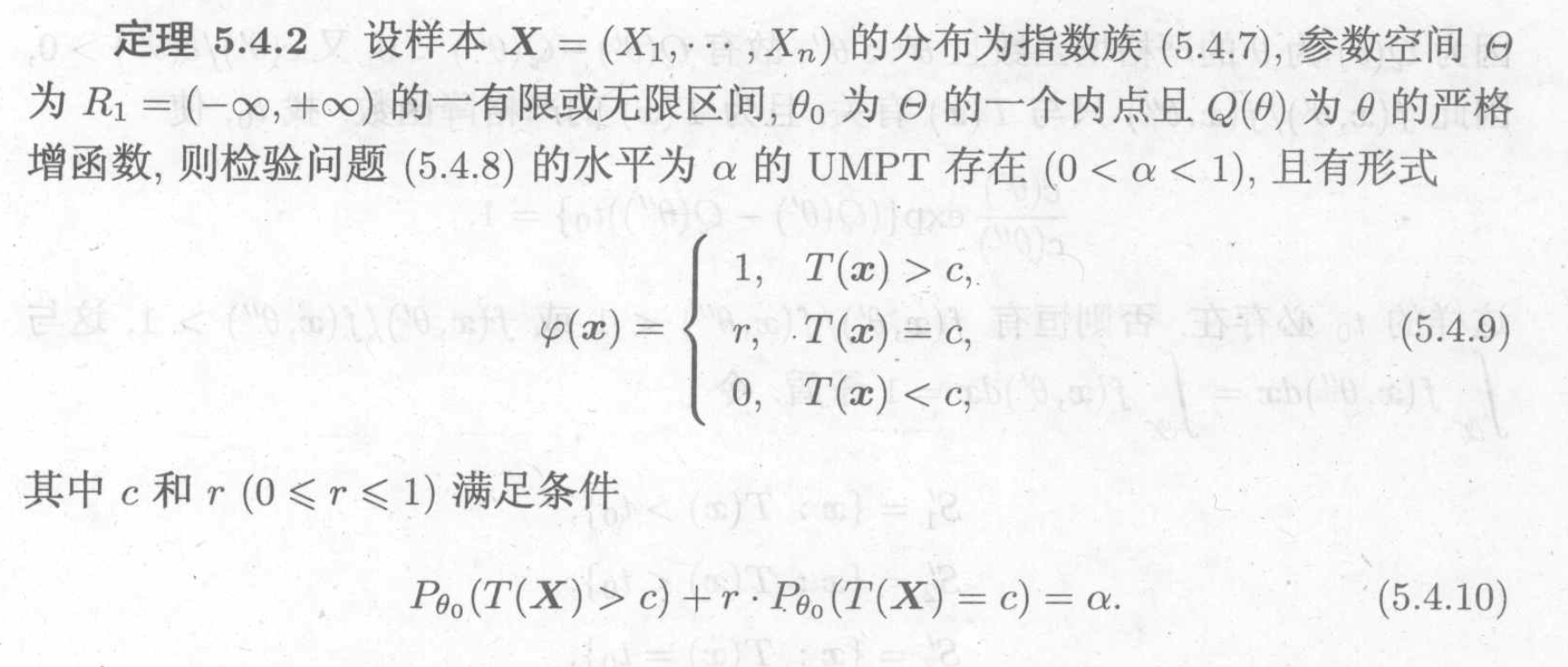
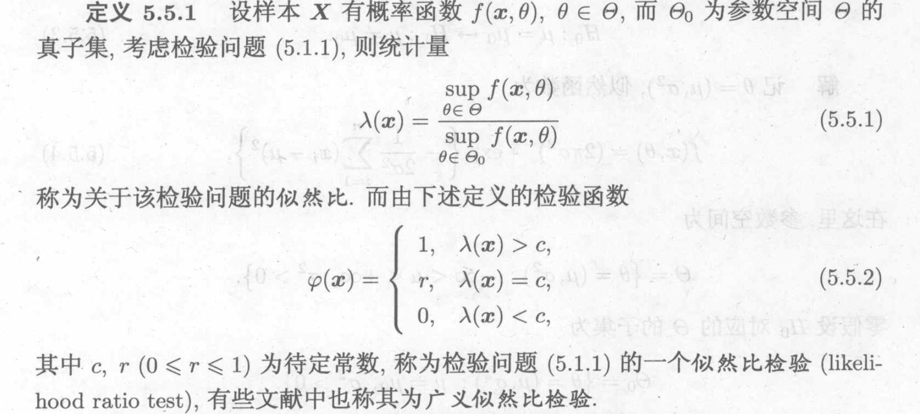
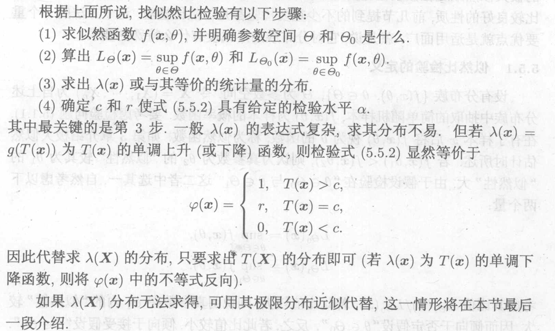
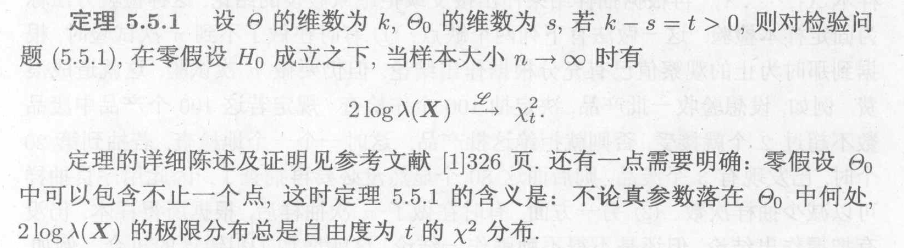
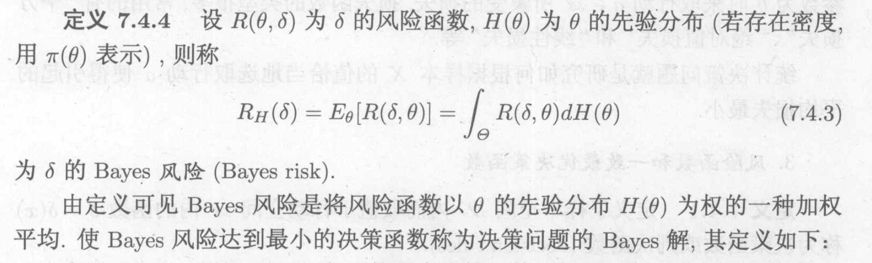
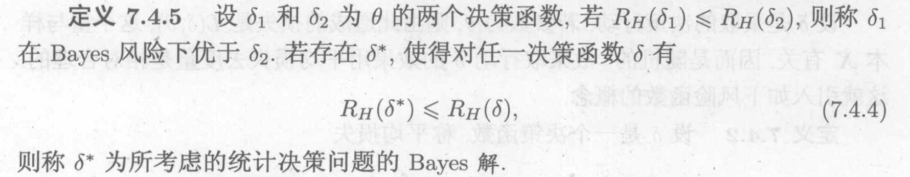
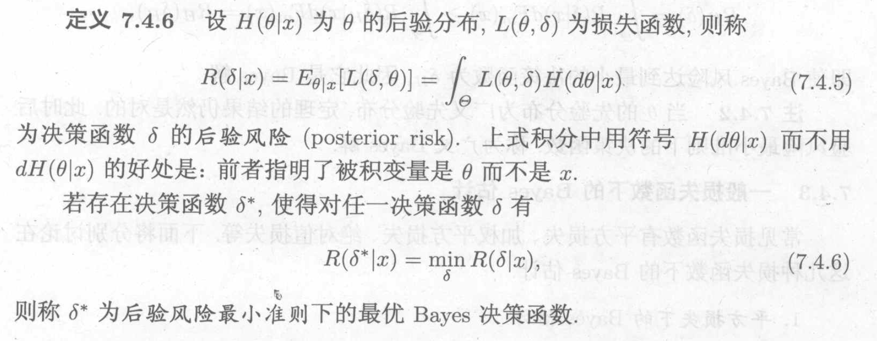
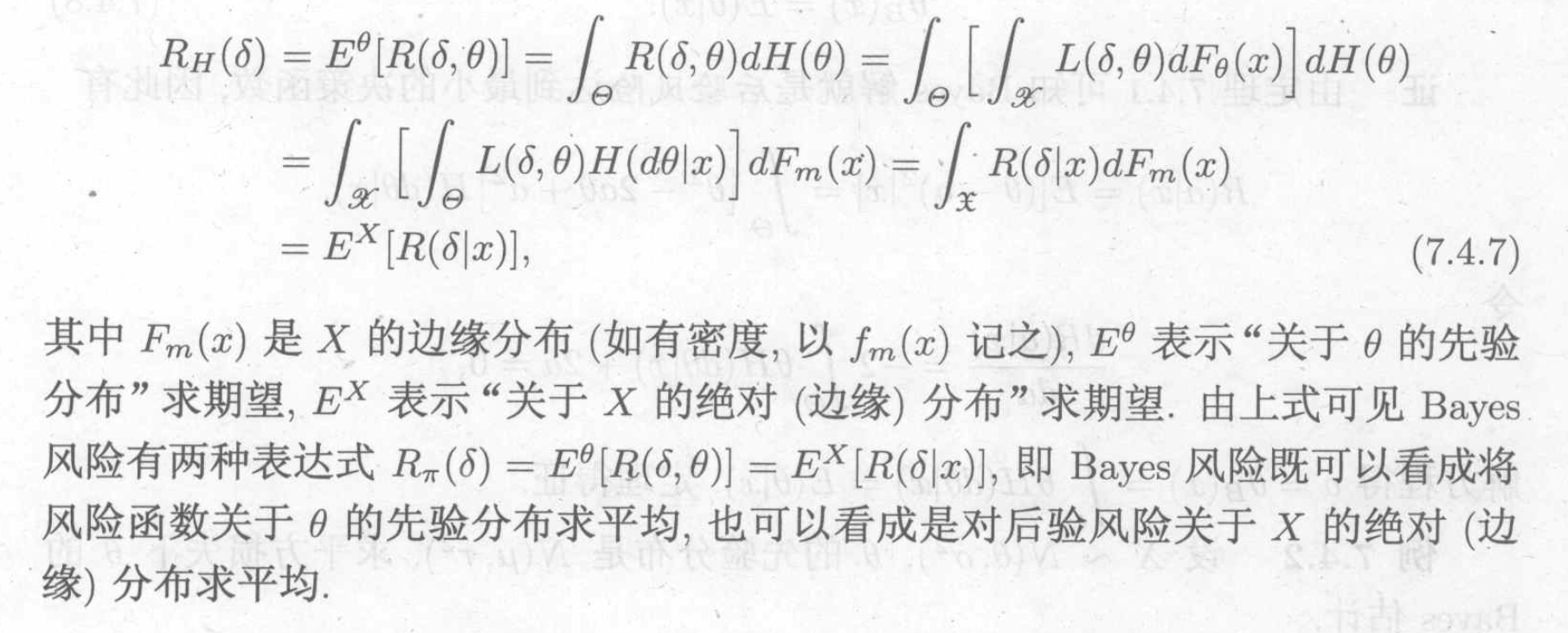
Numerical Statistics Course Slides Notes
1. sample space & stats
1.1. sample space
Def: sample space

Qua: => duality of sample space

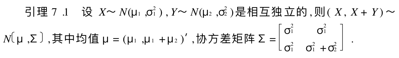
Def: iid

Def: parameter space

Def: distribution group

1.2. important stats
Def: statistic

1.2.1. single
1.2.1.1. sample mean
Def: sample mean

Qua: => mean & sum \[ \sum_{n=1}^{n}(X_i-\bar{X}) = 0 \]
Qua: => mean is the best for real mean

1.2.1.2. sample variance
Def: sample variance


Qua: => quatratic

1.2.1.3. sample covariance
Def: sample covariance

1.2.1.4. sample moment
Def: sample moment


1.2.1.5. U-stats
Def: U-stats (2-2)

Note:

Example: (2-2)

Example: (2-3)


Example: novel u stats (2-3)

Def: two-sample U-stats (2-3)

Example:

Qua: => variance of U-stats (2-3)

Proof:


(2-4)

Qua: => Var upper bound (2-4)

Qua: => asympototc normality (2-4)

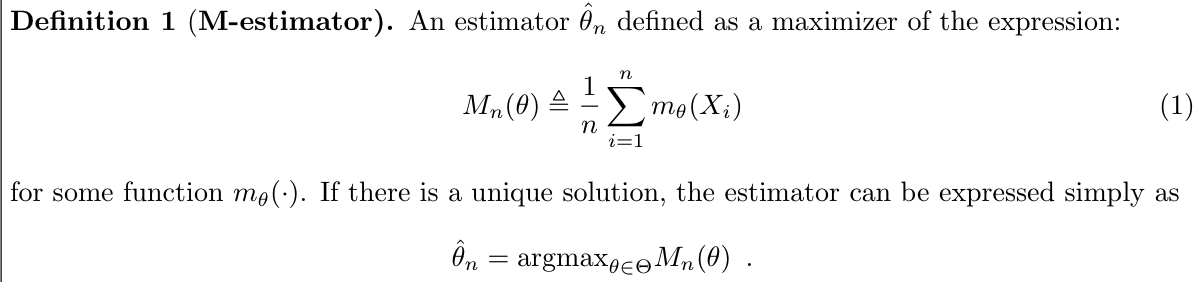
1.2.1.6. M-estimator and Z estimator
- Def: ULLN (2-9)

1.2.1.6.1. M-stats
Def: M-stats (2-9)
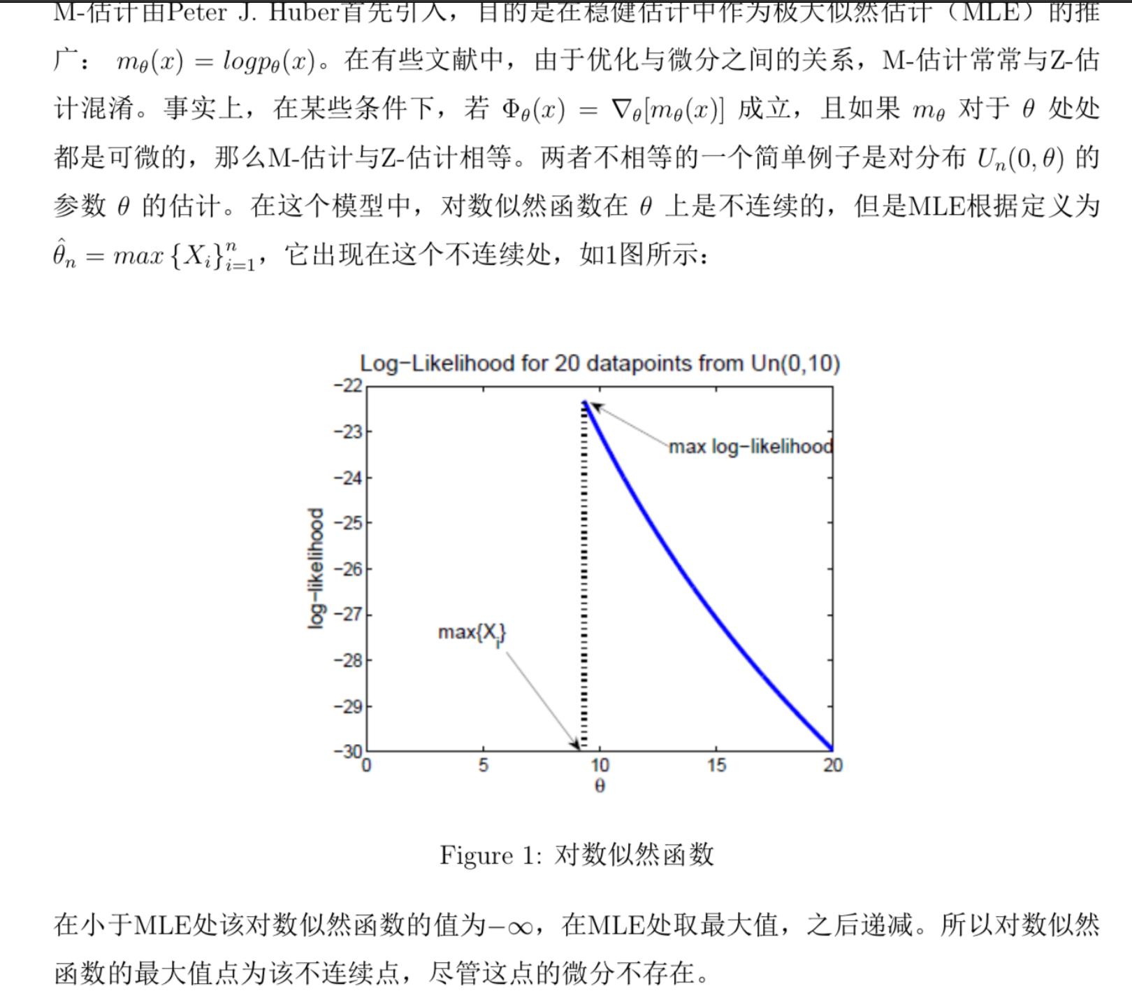
Note: Mstats and Zstats are not the same : use U() to prove, not differentiable => z do not exist on this point; but m is the largest on this point, so M & Z not the same.
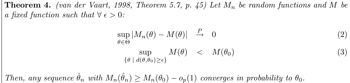
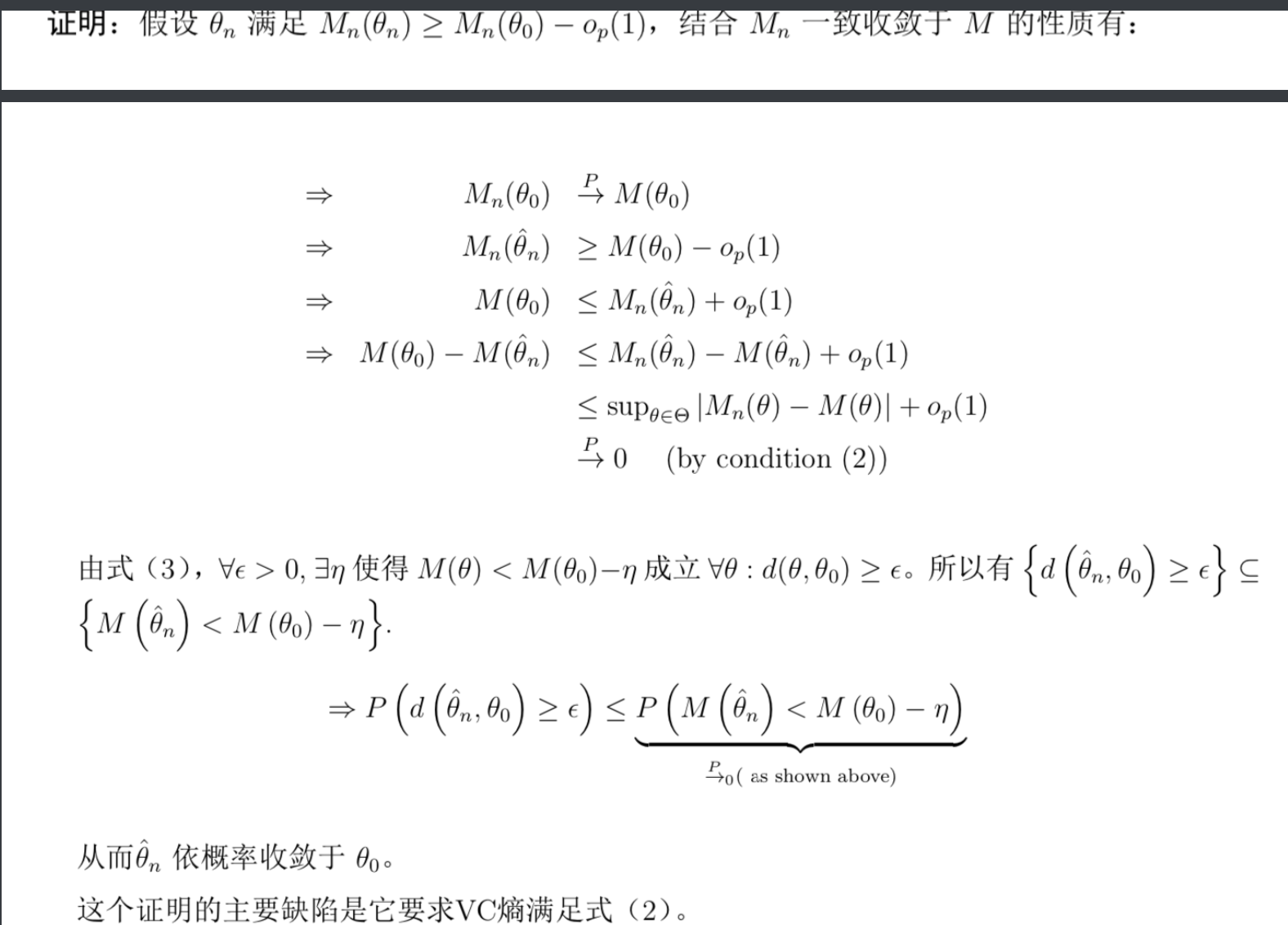
Theorm: => consistency of M stats
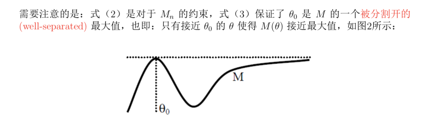
Usage: if M is uniformly consistent and have a well-separated maximum point, then we have sequence of \(\theta_n\) converge to \(\theta_0\)
Note: figure of the consitions
Proof:
1.2.1.6.2. Z-stats
Def: Z-stats (2-9)
1.2.1.7. order statistics
Def: order statistics

Qua: => distribution

Proof:

Note: when uniform(0, 1)

Qua: => joint distribution

Proof:

Note: when uniform(0, 1):

Def: sample median

Def: extremum of sample

Def: sample p-fractile

Def: sample range

Qua: distribution

Proof: using transformation trick

Note: when uniform (0, 1):

Proof:

1.2.1.8. sample coefficient of variation
Def: sample coefficient of variation

1.2.1.9. sample skeness
Def: sample skeness

1.2.1.10. sample kurtosis
Def: sample kurtosis

1.3. sufficient stats
Intro:


Def: suff stats

Theorm: element break, sufficient and necess condition

Qua: operation

1.4. complete stats
Def: complete stats

Qua: exp family & comp stats =>

Qua: => indepence & comp stats

Qua: operation

2. useful distributions
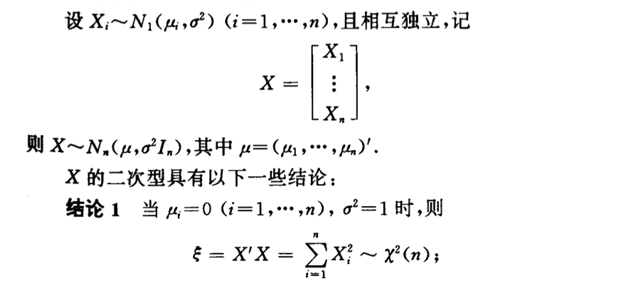
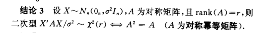
2.1. exp
Qua: => x2

2.2. gaussian
2.2.1. distribution
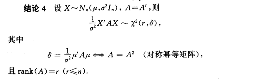
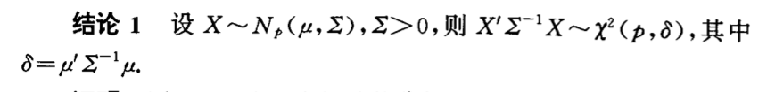
Qua: => X2

Qua: operation


2.2.2. stats & estimation
2.2.2.1. stats
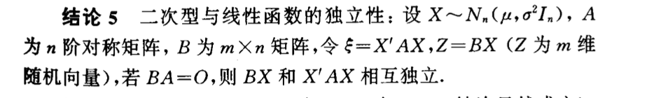
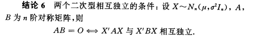
Qua: mean & variance => independent

Proof: see book
Qua: Mean/Variance => distri

Qua: Mean-Mean/Variance => distri

Qua: Variance/ Variance => distri

2.2.2.2. estimation
2.3. X2
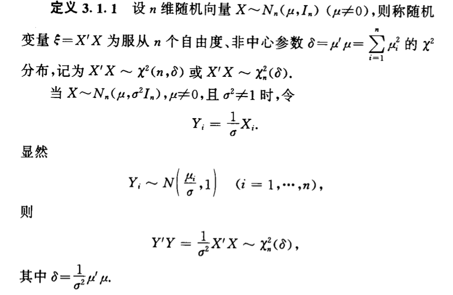
Def: central X2 distribution

Qua: => pdf

Proof: transformation, see book
Note:


Qua: => special & operation

Def: non-central X2

Qua: => pdf

Proof:

Qua: => distri & operation

2.4. gamma
Def: gamma distribution

Qua: gamma => X2

2.5. t
Def: central t distribution

Qua: pdf

Proof:

Note:

Qua: => E & Cauchy

Def: non-central t distribution

Qua: => pdf

Qua: => E, D

2.6. F
Def: F stats

Qua: => pdf

Proof:

Note:

Qua: => special & operation

Proof:

Def: non-central F


Qua: => pdf

Qua: => special & X2

2.7. exponential family
Def: exponential family
(Gaussian, +-Bio, Posson, Exp, Gamma)

Qua: => all distribution have same support set

Def: natural form & natrual space

Qua: => under natural form , natural space is Convex Set

Qua: => analytical stuff


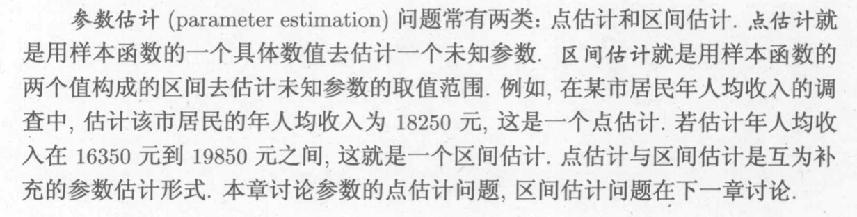
3. parameter estimation (usage of stats)
Def: parameter estimation
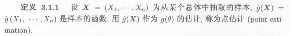
3.1. point estimation
Def: point estimation
3.1.1. quality of estimation
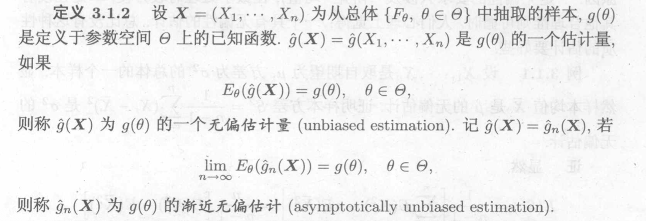
Def: unbiased estimation
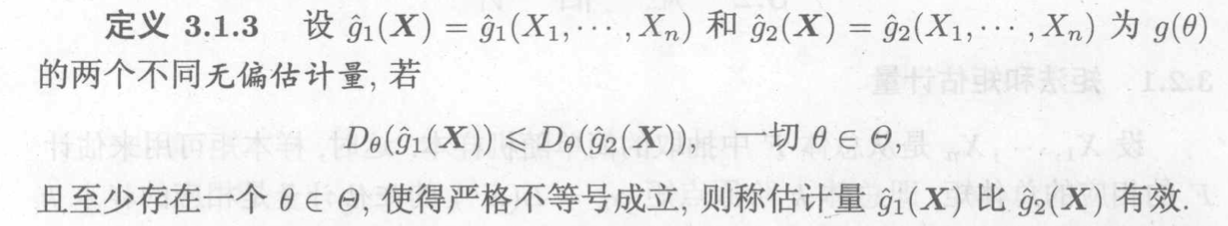
Def: efficiency
Def: consistency
(book)

(2-?)

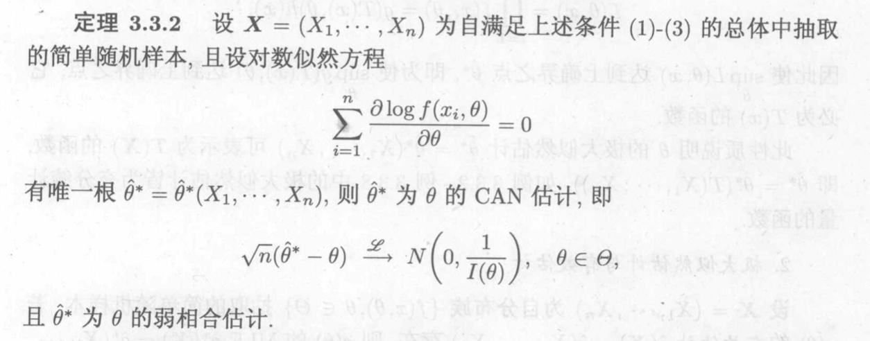
Def: consisten asymptotic normal estimation
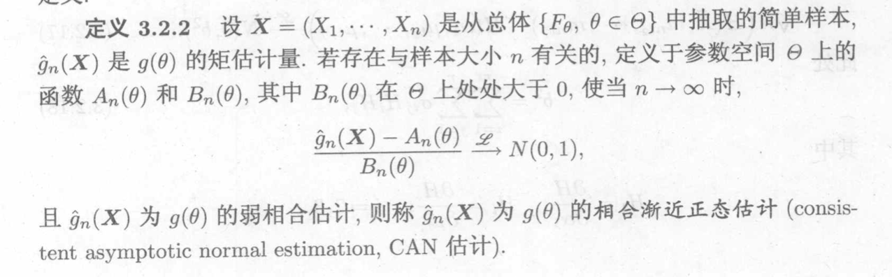
Note: both consistent & Gaussian

unbiased consistent gaussian(CAN) f_operation sufficient complete moment cond cond cond yes no no mle no cond cond yes yes umvue yes
3.1.2. moment estimation
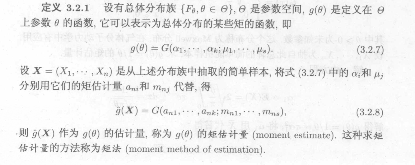
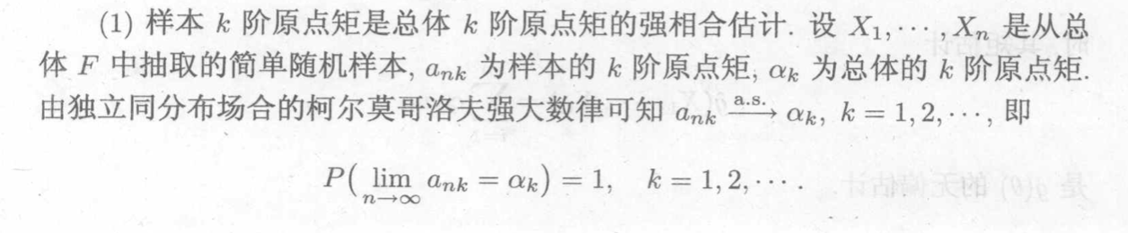
Def: moment estimation
Usage: estimate \(\theta\) => turn \(\theta\) to \(f(moment, moment)\) => turn to \(f( \hat{moment}, \hat{moment_est})\)
Qua: => normally biased, sometimes not biased

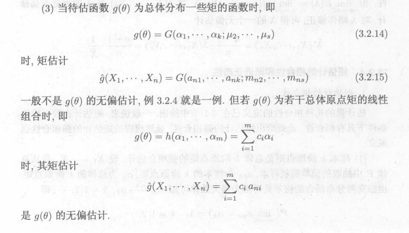
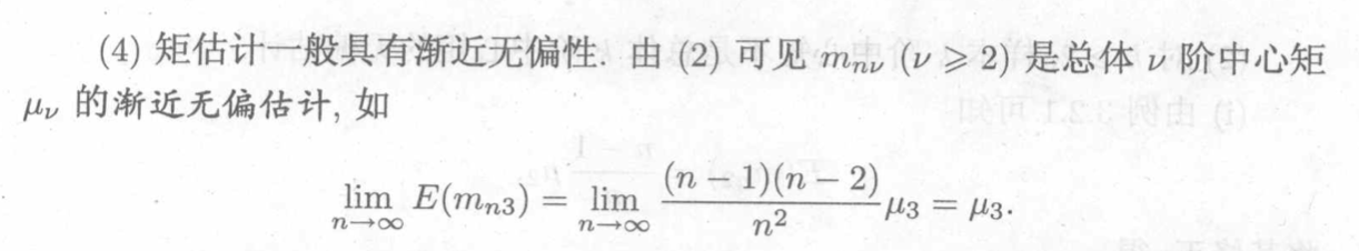
Qua: => strong consistency

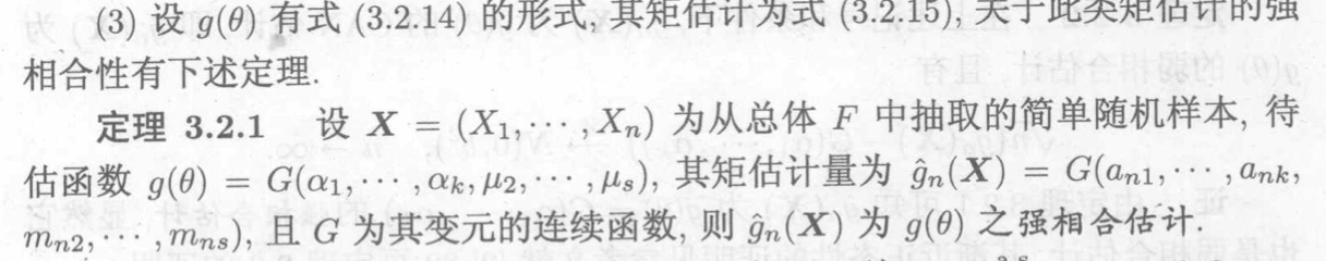
Qua: => CAN
Usage: normal situation
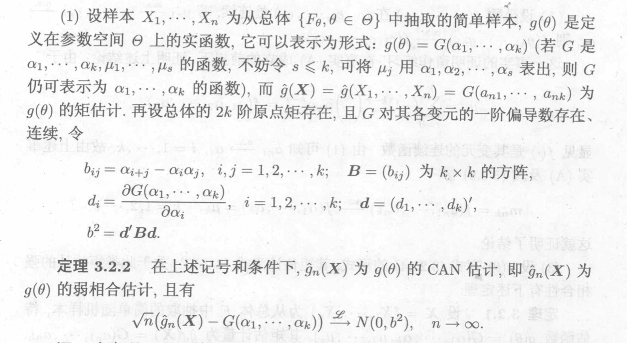
Qua => CAN
Usage: when \(\theta\) can be expressed with 1/2 central moment
3.1.3. mle estimation
Def: likelihood function
Note: this is the same as pdf, only in pdf x is variable, in likelihood \(\theta\) is variable.
3.1.3.1. parameter
Def: MLE (parameter), usage of M-estimator
Usage: given x & likelihood function, seek for \(\theta\) to make likelihood function the largest .
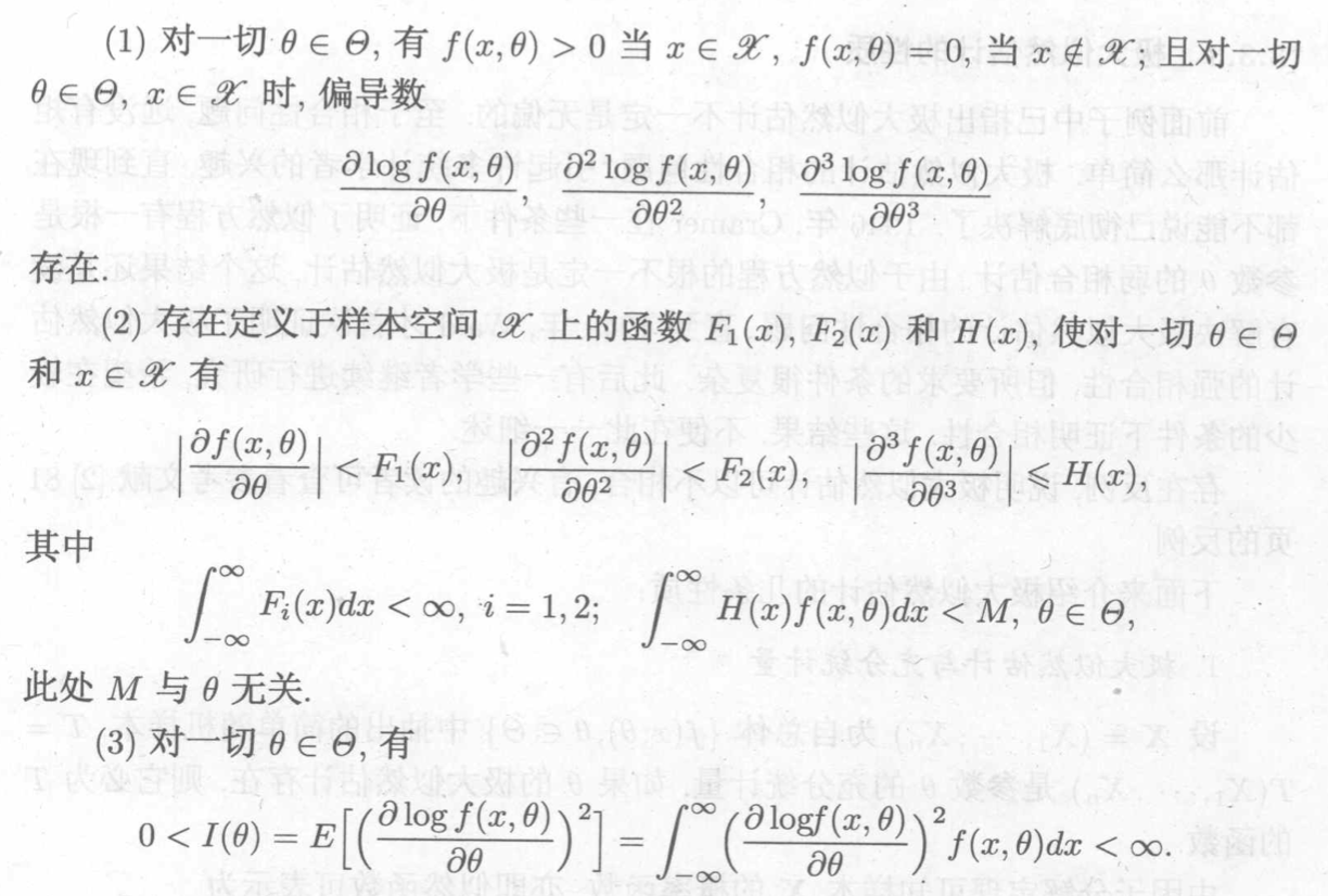
Theorem: conditions to make MLE solvable =>
Corollary: when distribution
Corollary: when distribution is exp family =>
Proof:
Qua: => sufficient stats
Qua => CAN
3.1.3.2. non-parameter
Def: MLE (非参数)(2-9)

Note: 因为是非参,所以需要求积分。(2-9)

Note:小于等于0因为这是KL散度的形式p0其实和p一回事。
Qua: p0 and MLE(pn)'s KL distance (2-9)

3.1.4. umvue
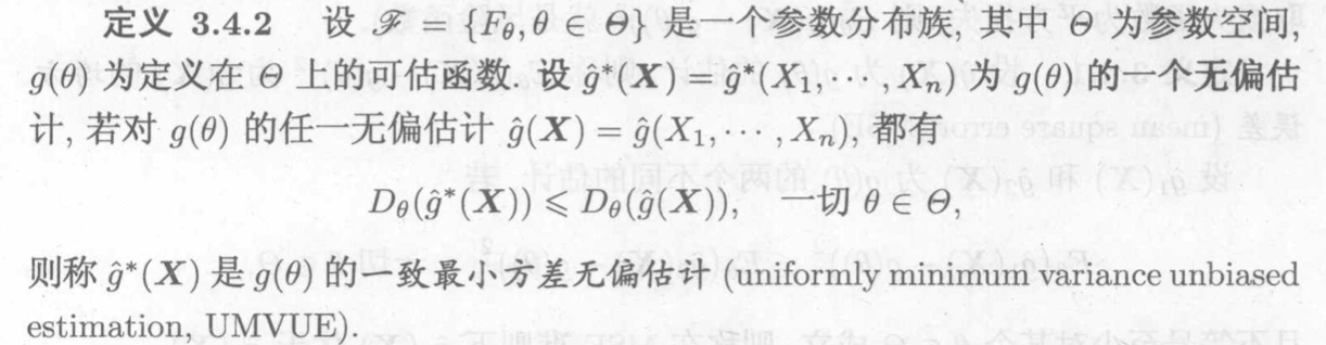
Def: estimatable function
Def: min MSE
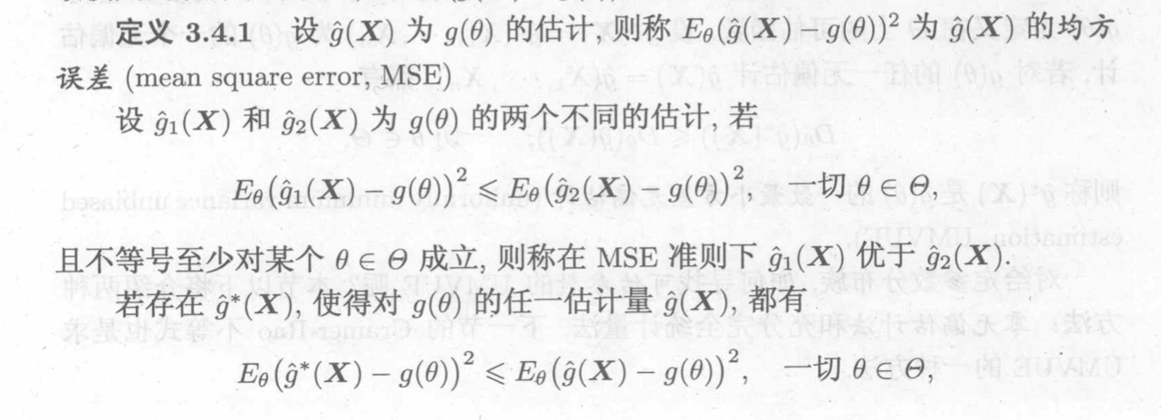

Def: min Var & unbiased (UMVUE)
Usage: sometimes we can not find min MSE since the realm is too large, we can make it smaller by constrain it in unbiased family, and min -Var + unbiased = min MSE.
Lemma: => smaller Var
Usage: the lemma give us a hint to make Var smaller from an biased estimate by doing a conditional expectation on a sufficient stat.
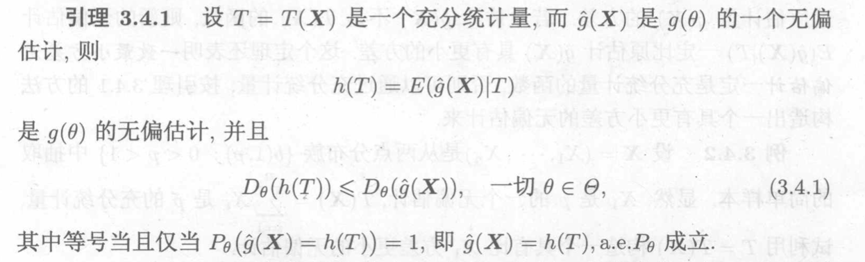
Note:
3.1.4.1. 0-unbiased estimate
Theorem: Cov, E =>
Usage: sufficient condition for UMVUE
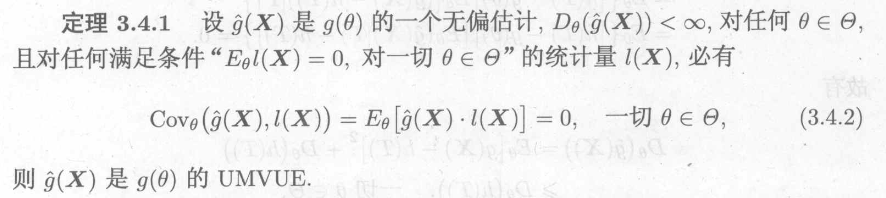
Note: we can't use this to construct a UMVUE, but we can 验证 if it is.
3.1.4.2. sufficient & complete estimate
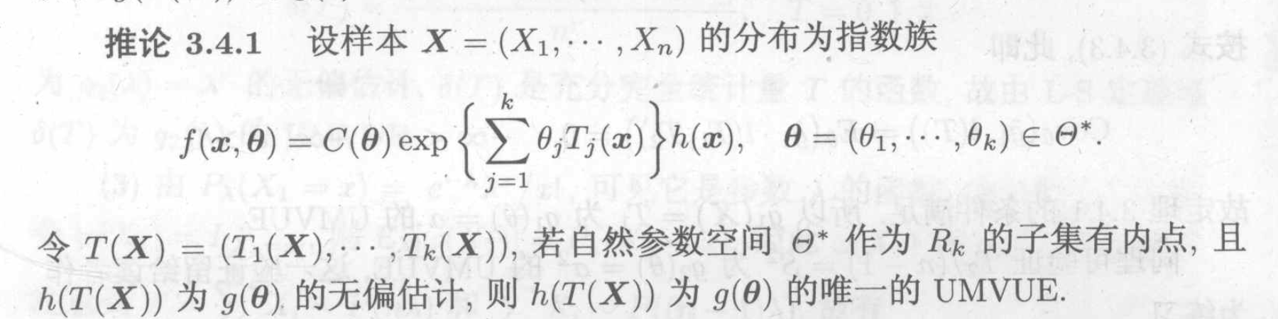
Theorem: Lehmann - Scheffe, suff & complete =>
Corollary: exp family =>
#### CR inequality estimate
Intro: what is and why we need CR: it is a tool to determine if a stat is UMVUE.
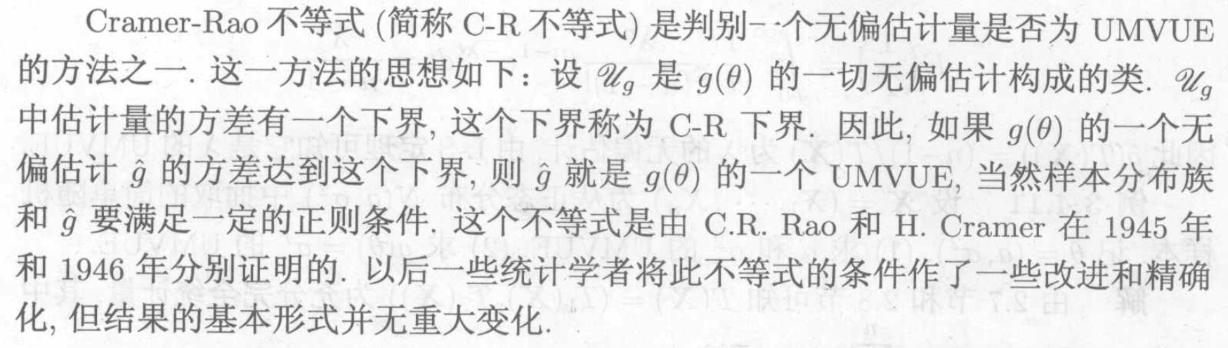
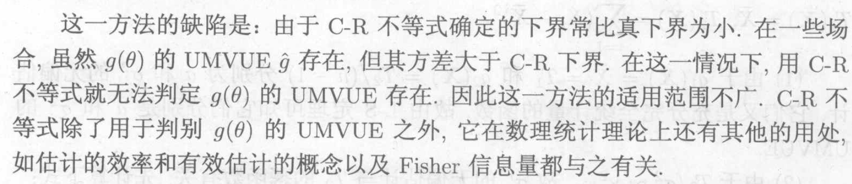
Note: cons of CR
3.1.4.2.1. singular parameter
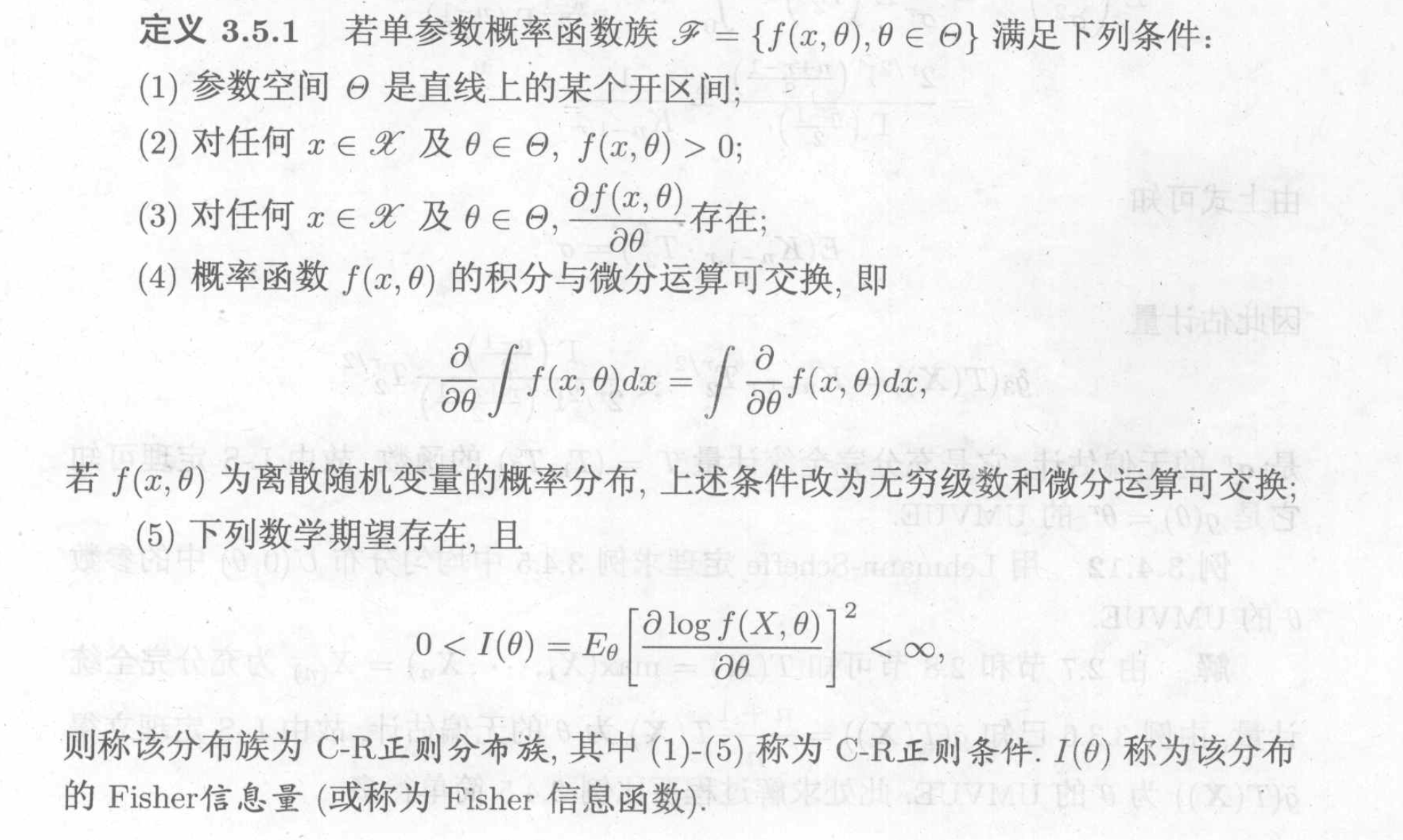
Def: CR regular family
Def: CR inequality
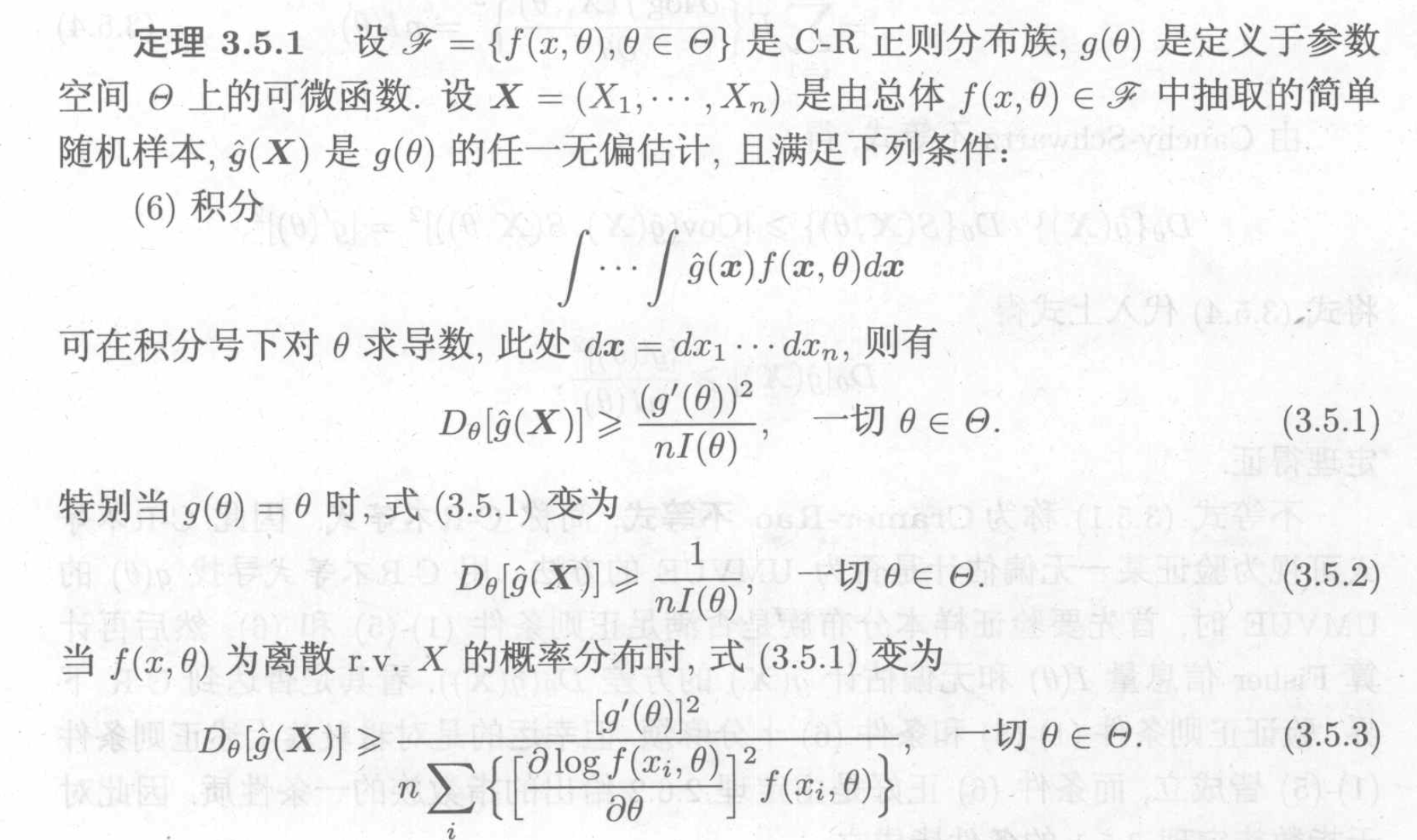
Note: CR can be viewed as a tool for 验证 ·UMVUE.
Theorem: cases of exp family =>
Note:

Theorem: despite exp family, when will C-R reach equation =>
Note:
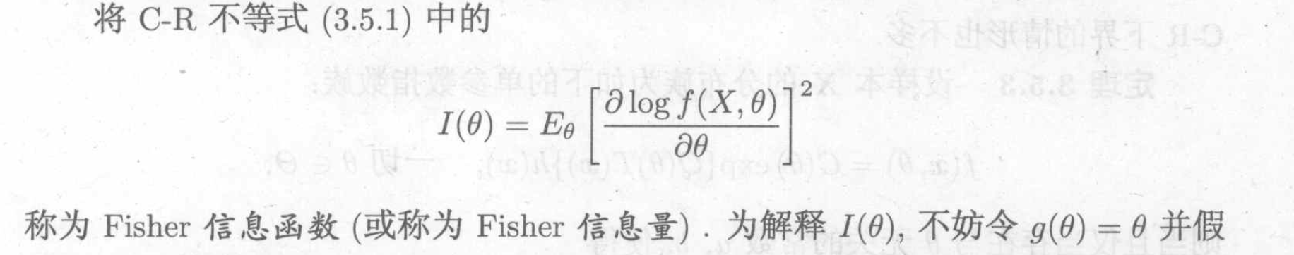
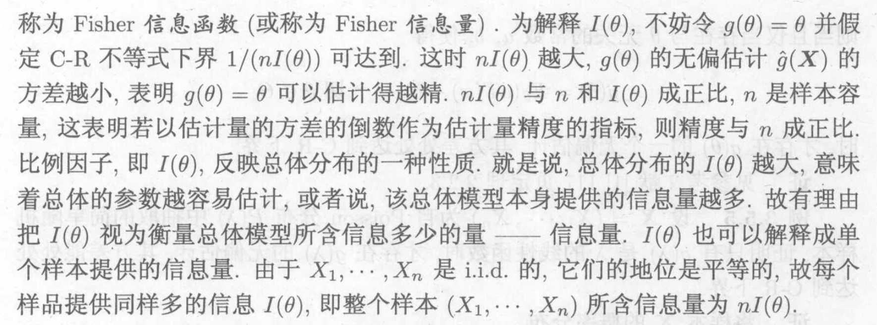
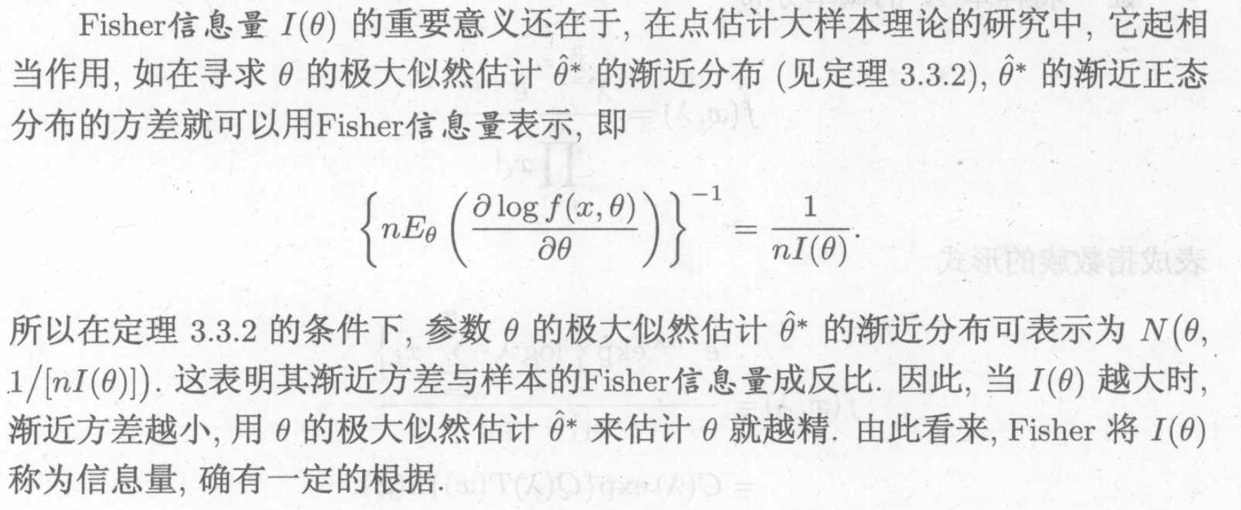
Def: fisher information function ( for a distribution )
Note: the larger \(I(\theta)\), the easier is X to estimate its parameter, the more information the model itsself provides.
Note: fisher function in the law of large number.
3.1.4.2.2. multi parameter
P120
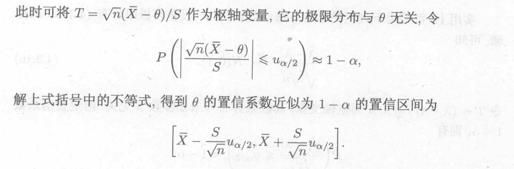
3.2. interval estimation
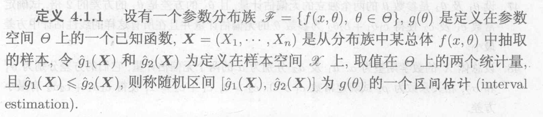
Def: interval estimation
Usage: the range of possible $ $
3.2.1. quality of invertal estimation
Def: confidence coefficient
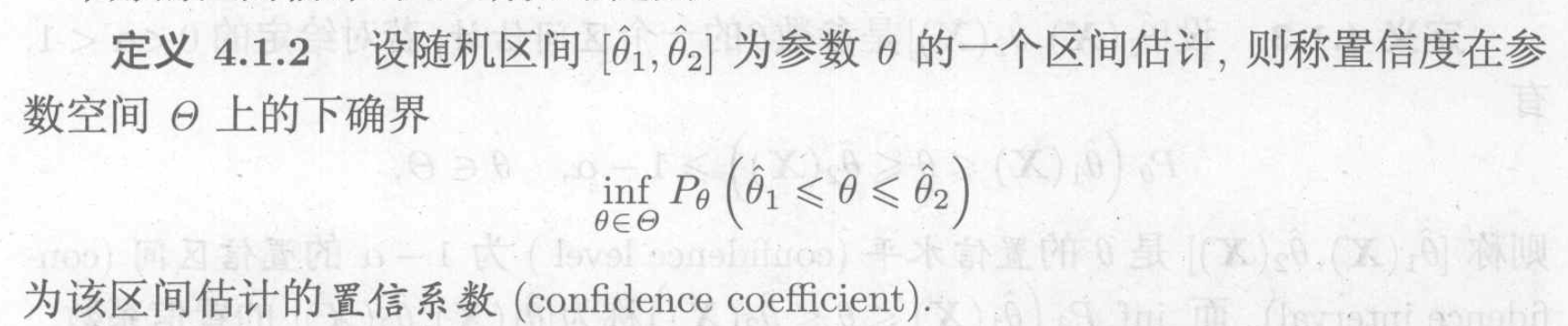
Note: the larger the better
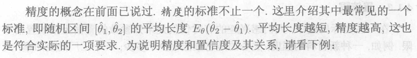
Def: length (precision)
Note:
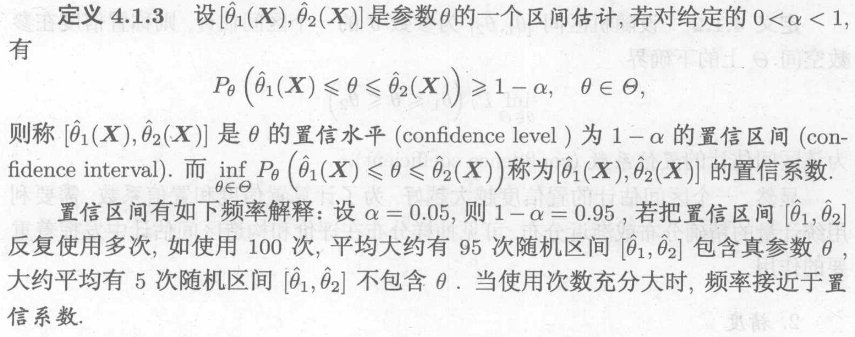
Def: condidence interval
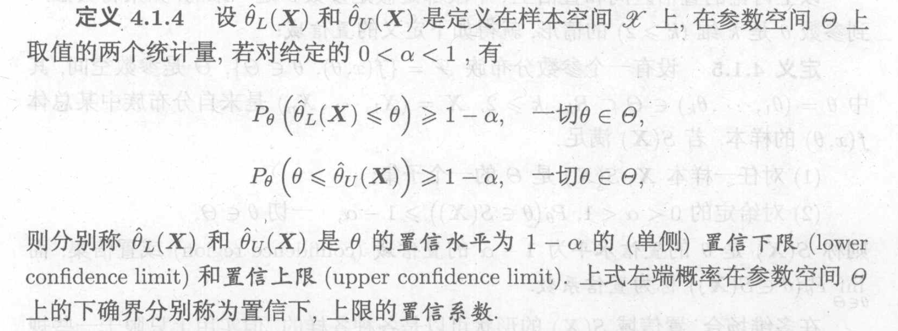
Def : lower confidence limit
Note:
Theorem: relationship with interval
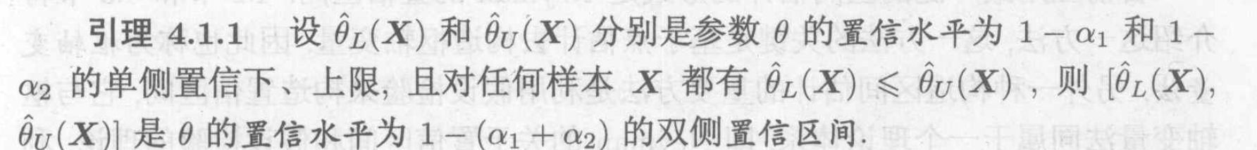
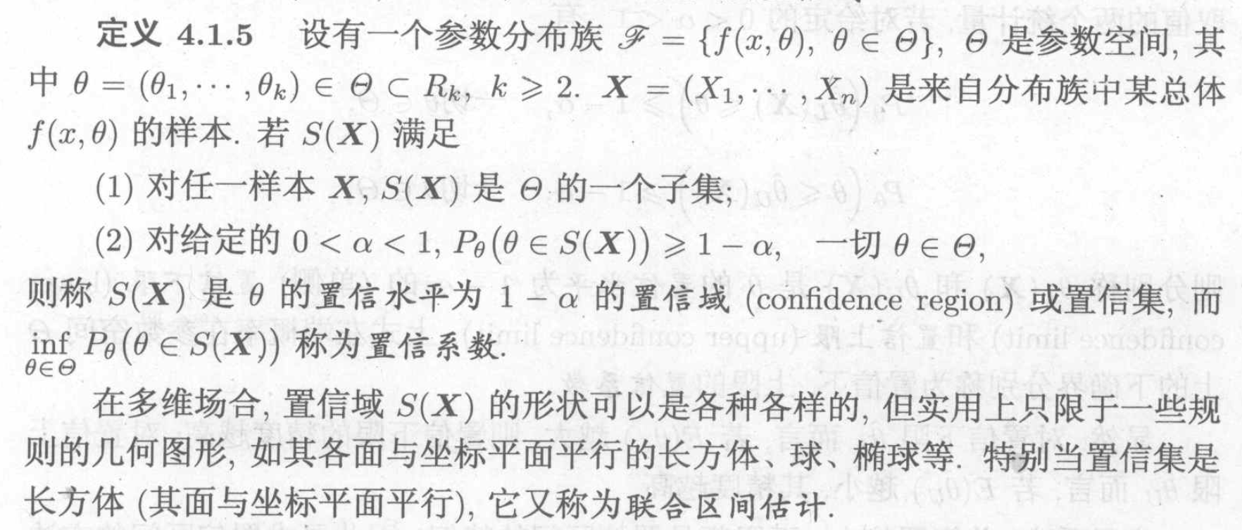
Def: >1 dimension interval, confidence region
3.2.2. Neyman estimation
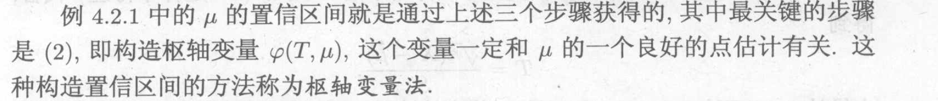
Algorithm: from point estimation to interval estimation
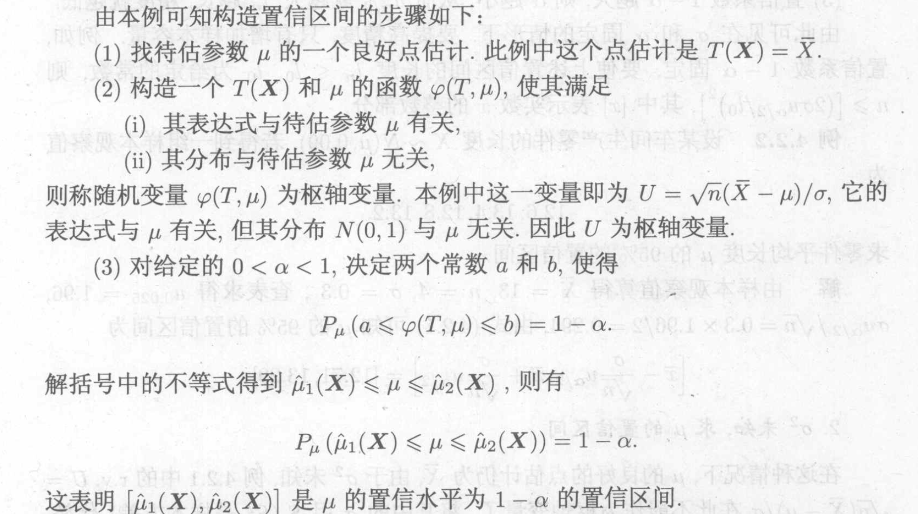
Note:
3.2.2.0.1. small sample method
Example: Gaussian
see slides P129
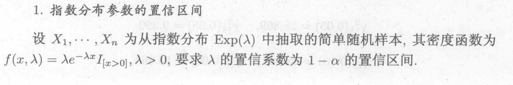
Example: exp
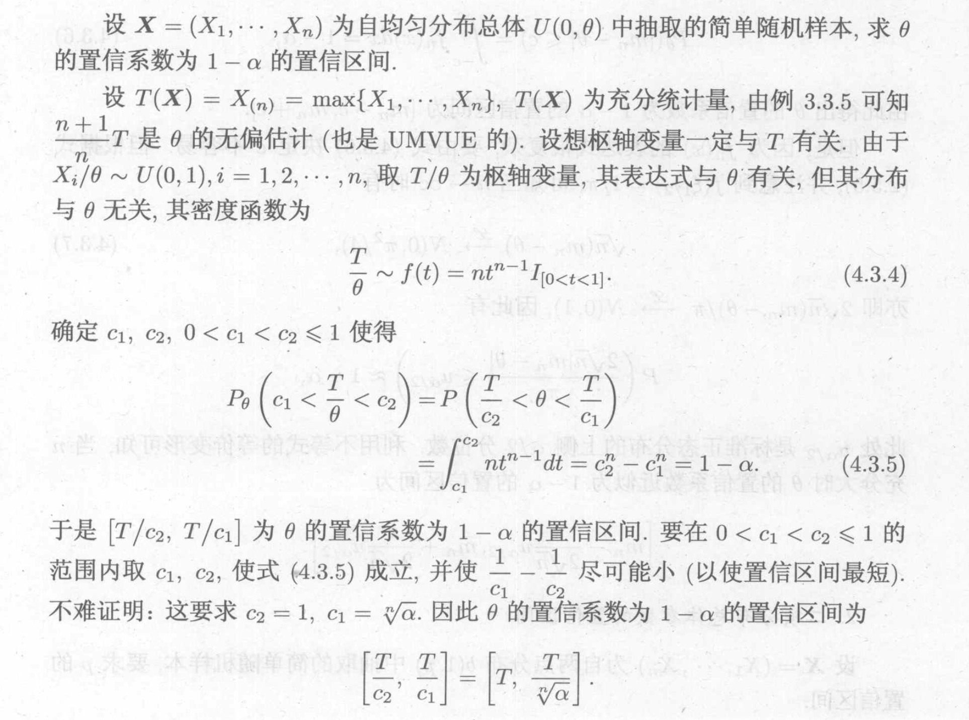
Example: uniform
3.2.2.0.2. big data method
Using big data distribution estimation to get a Neyman interval estimation.
Example: Caughy
Example: bionomial distribution
P142
Example: Possion distribution
P143
Theorem: general methods
Usage : using MLE & information function to approximate distribution
Theorem : no parameter case, when we can't use parameter to construct MLE .
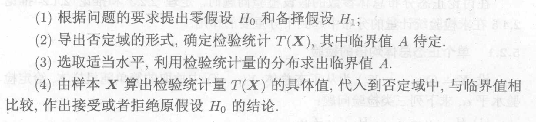
3.2.3. hypothesis
3.2.4. Fisher estimation
P143
3.2.5. Tolerance estimation
P15
###Bayes estimation
4. hypothesis test
4.1. parameter hypothesis
Def: parameter hypothesis
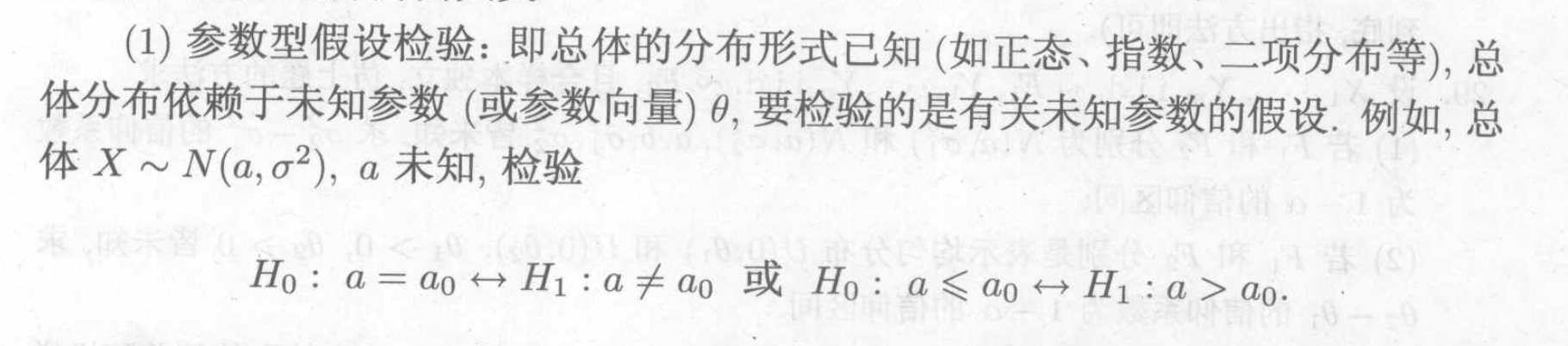
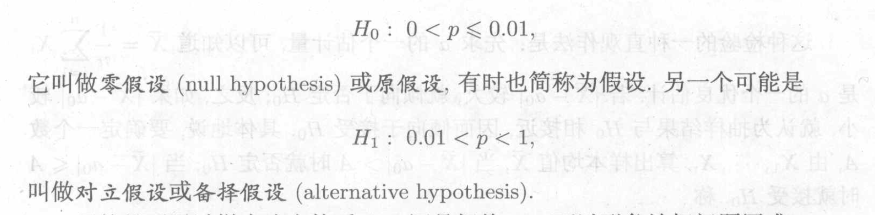
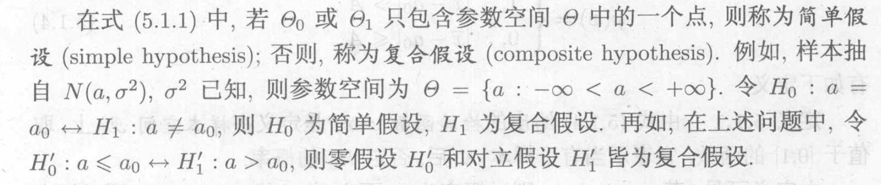
Def: null hypothesis & alternative hypothesis
Note:
Def: reject region & accept region
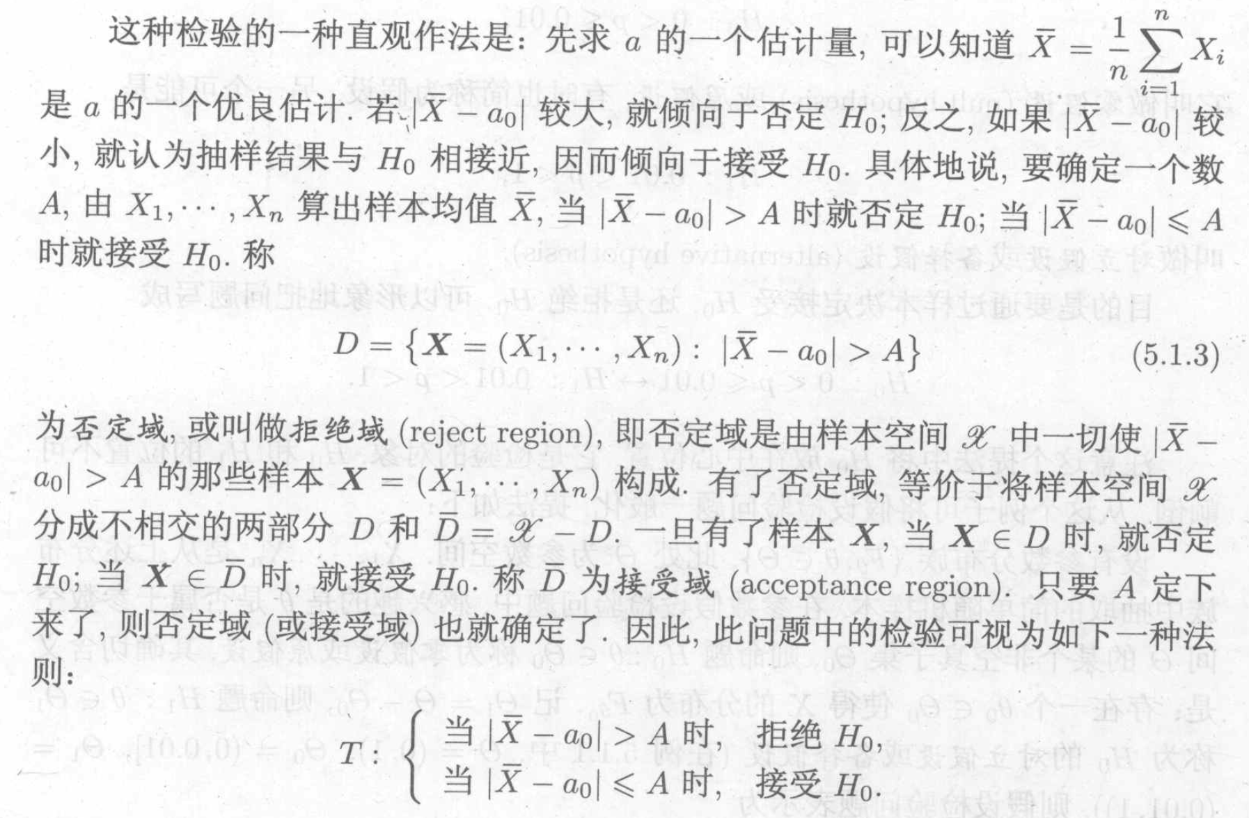
Def: 检验函数
Usage: when we decline H0
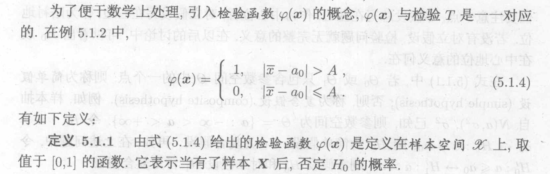
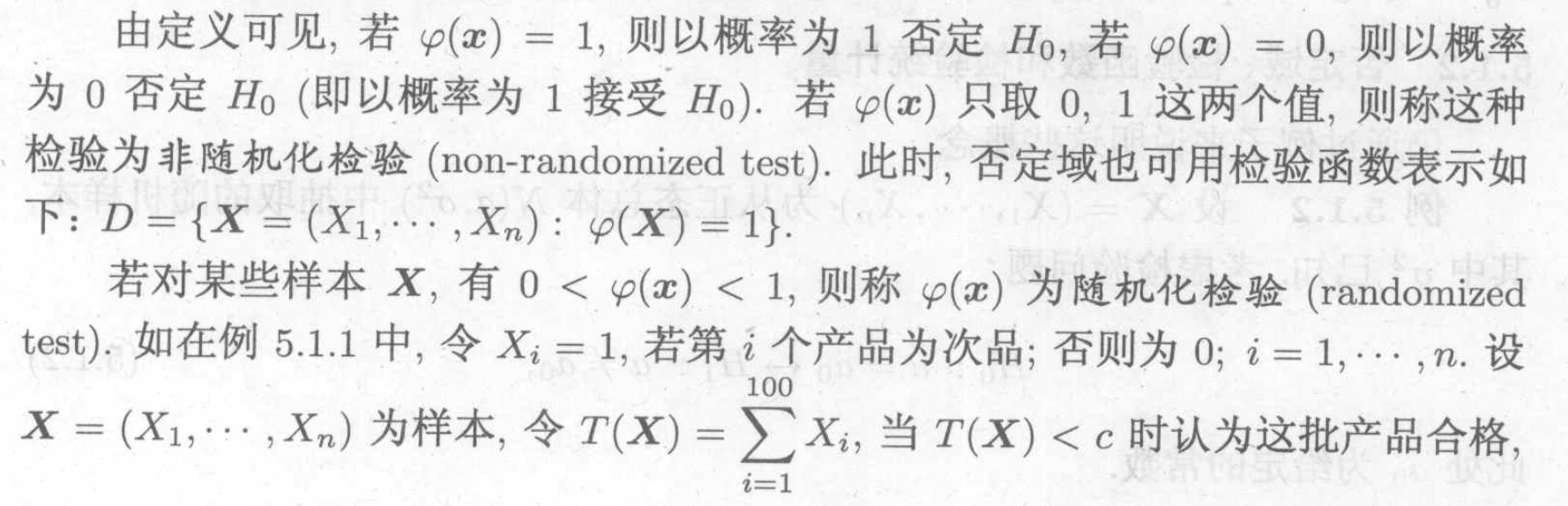
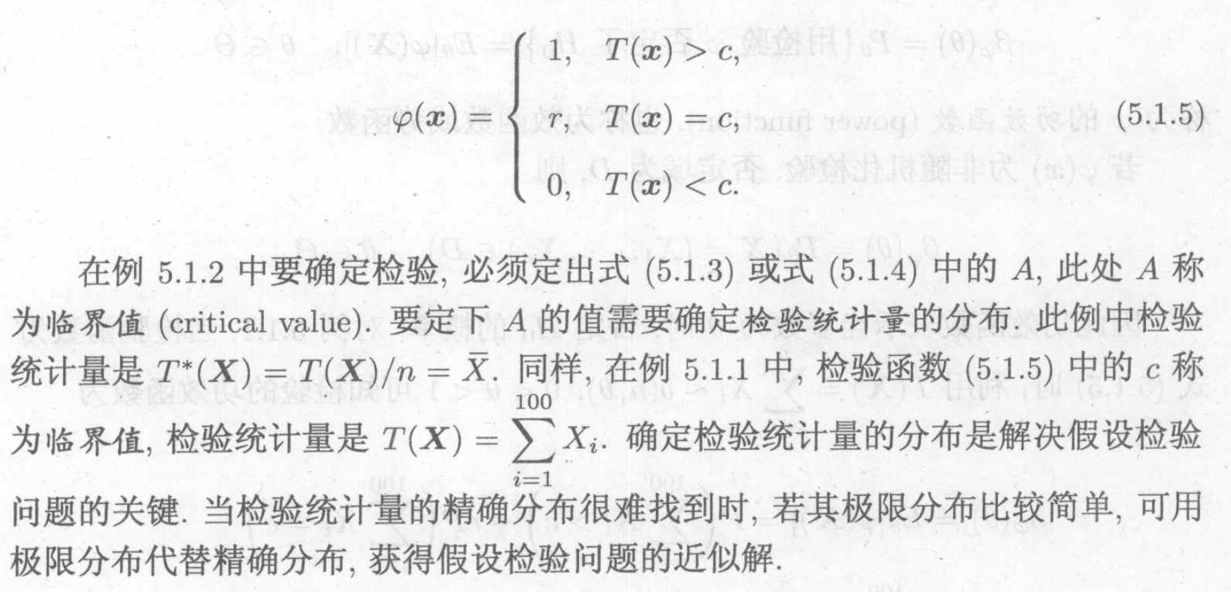
Def: randomized test
Def: critical value
4.1.1. two types of error
Def: two types of error
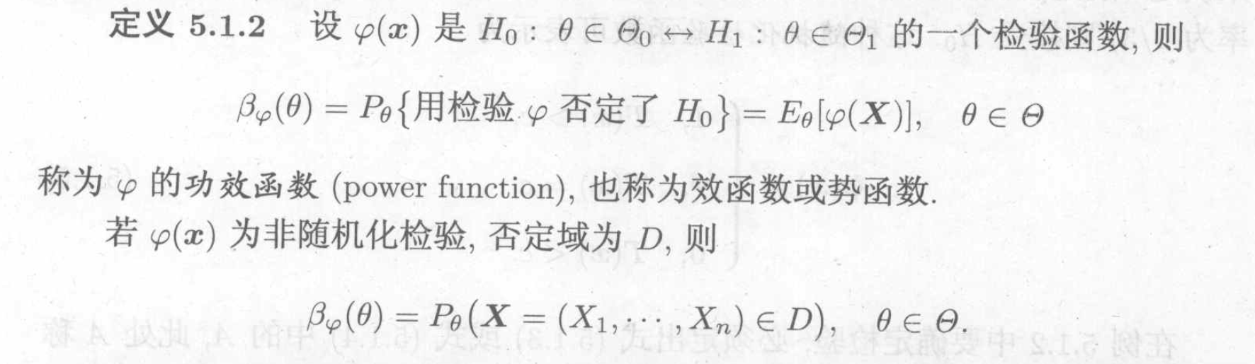
Def: power function
Note: when \(\theta\) is fixed, the possibility we decline H0

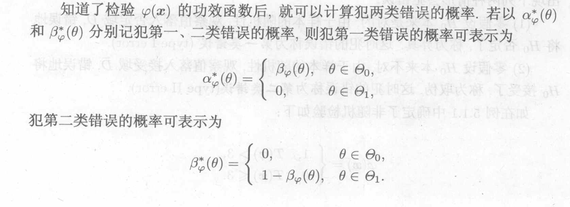
Note: using power function to indicate two types of error.
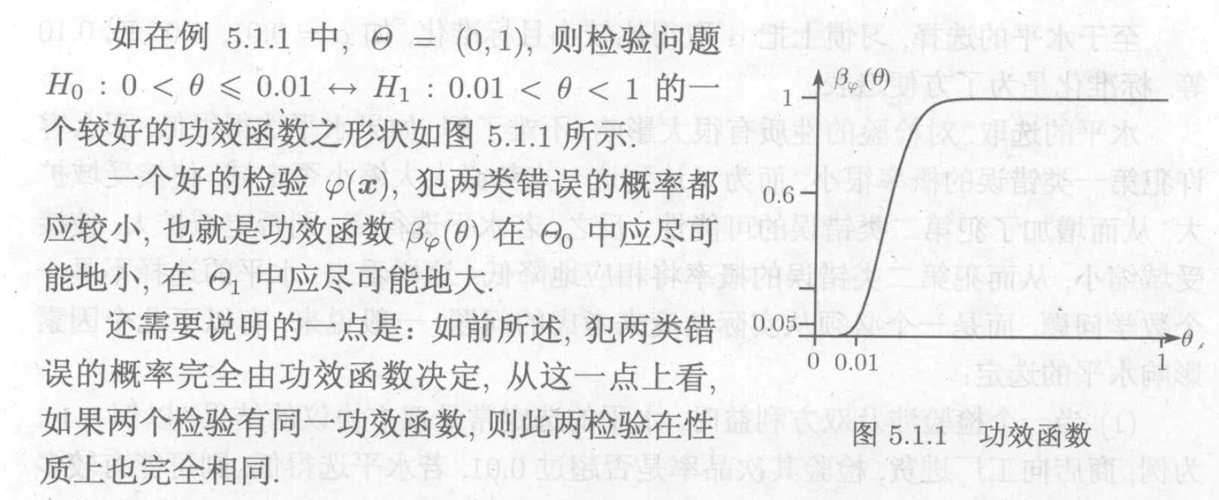
Note: figure of power function
4.1.2. Neyman-Pearson protocal
Def: Neyman-Pearson protocal
Note: first consider first type of error then second, we set H0 as solid hypothesis, we don't consider it wrong unless necessary.
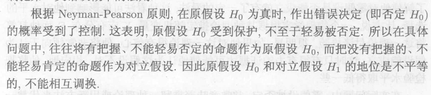
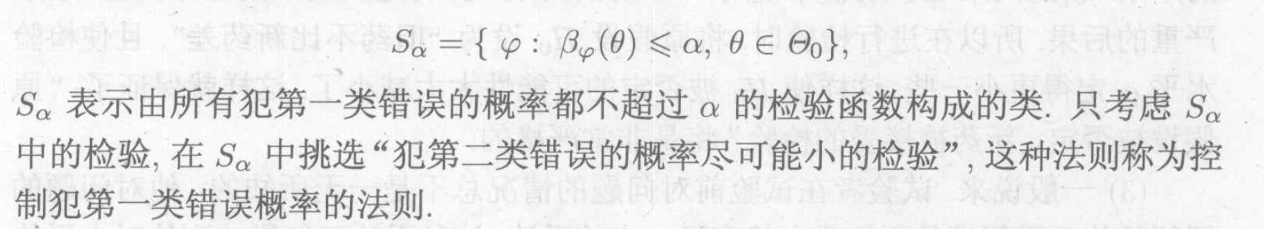
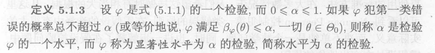
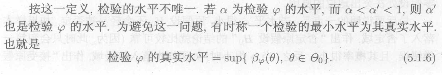
Def: level of hypothesis
Note: how to set the level

4.1.3. general test
Def: general methods
Example: Gaussian
P170
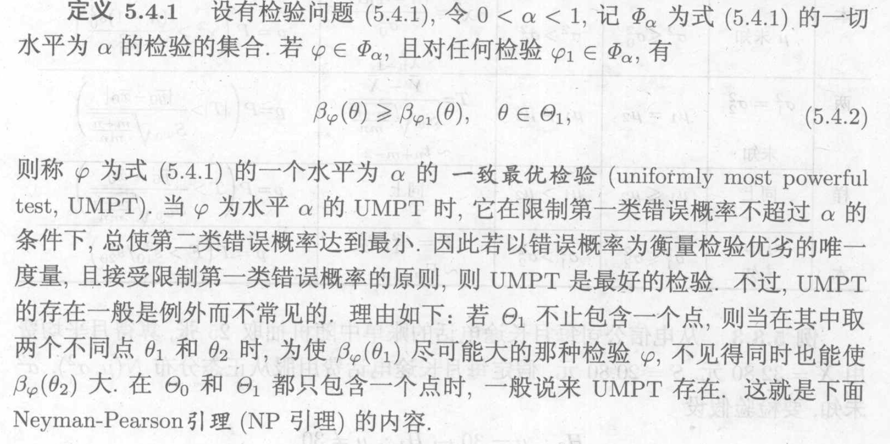
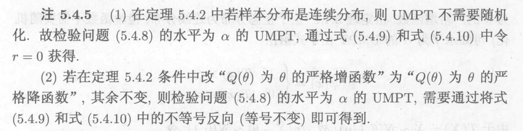
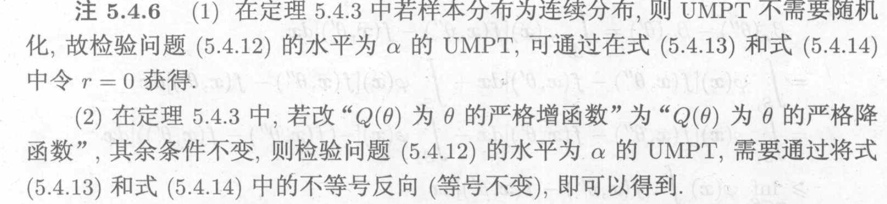
4.1.4. uniformly most powerful test(UMPT)
What is the best way to do test?
Def: UMPT
Theorem: NP theorem existence of UMPT =>
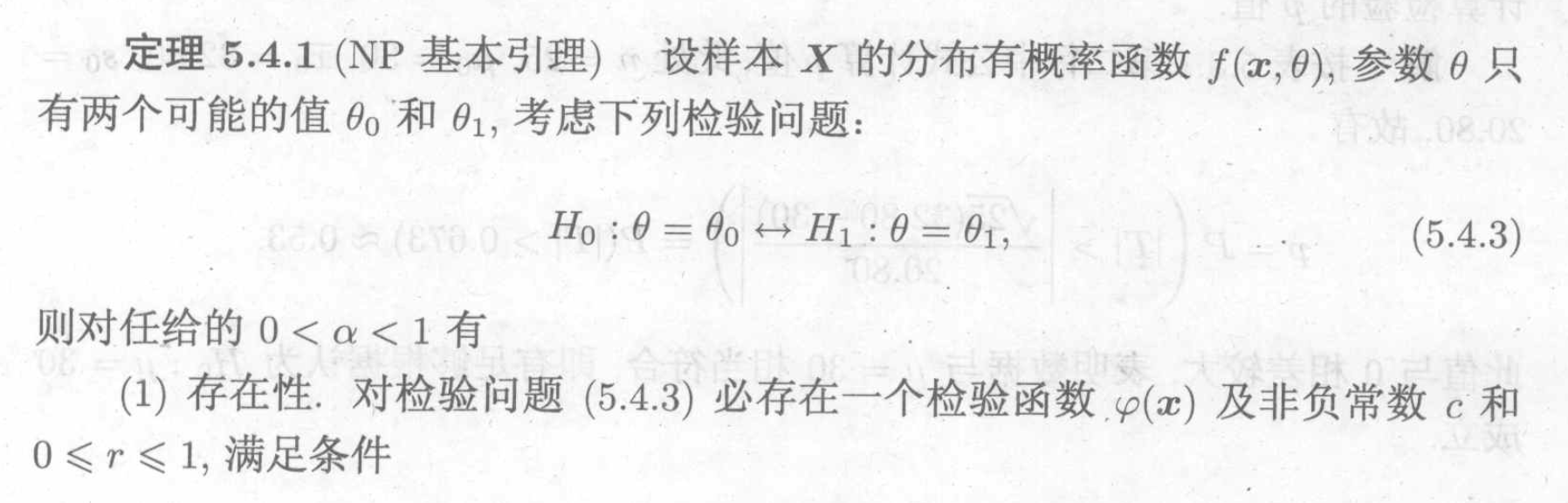
Note:
Note:
Intro:
Theorem: for the above special hypothesis, we have UMPT =>
Note:
Intro: a reversed version also exists
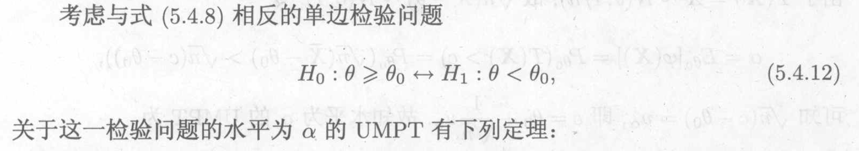
Theorem: for the above special hypothesis, we have UMPT =>
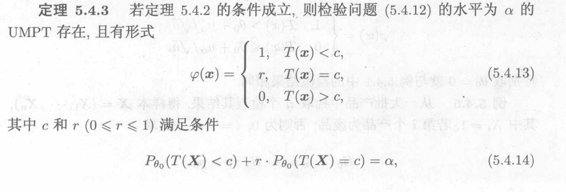
Note:
4.1.5. likelihood ratio test
Def: likelihood ratio test
Algorithm:
Theorem: => distribution estimation
4.1.6. sequential probability ratio test
Def: SPRT

4.2. non-parameter hypothesis
4.2.1. sign test
P234
4.2.2. signed rank test
P238
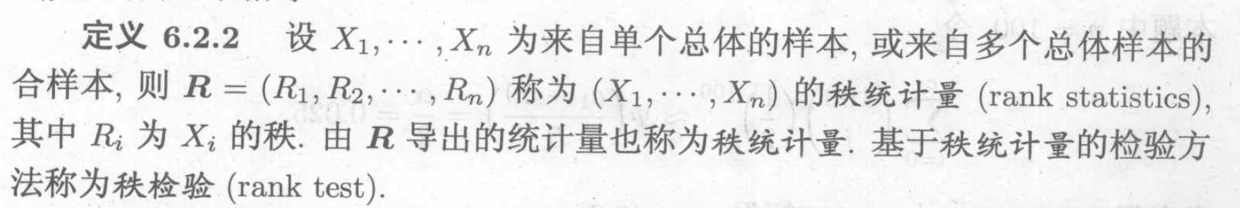
Def: rank
5. Bayes method
Def: prior distribution
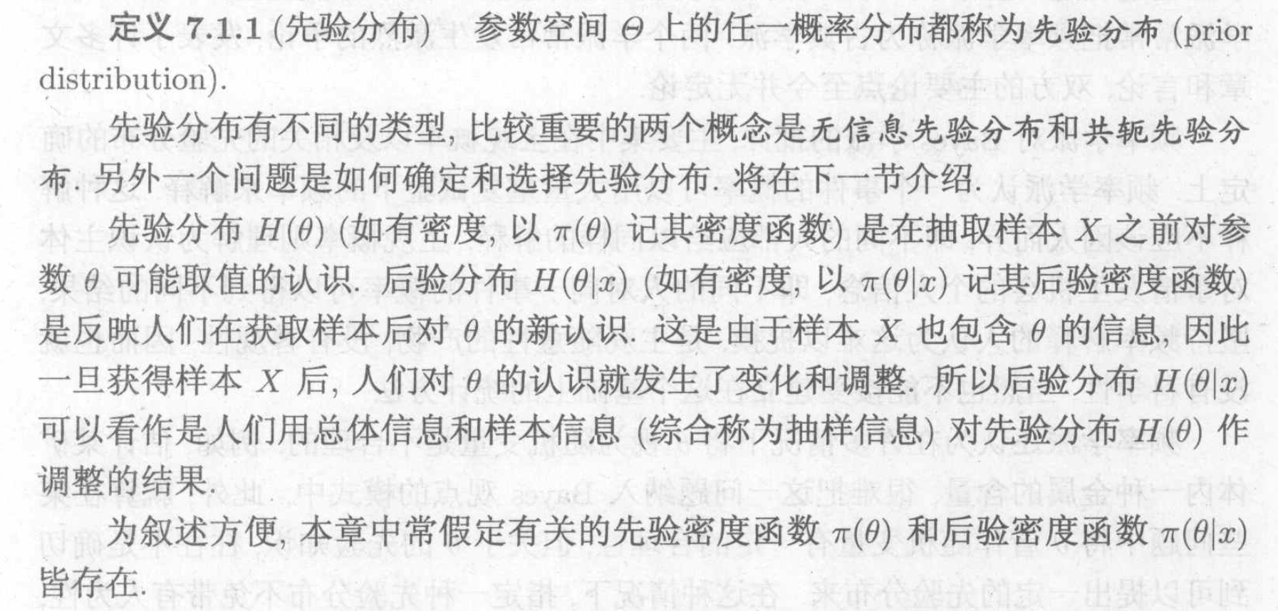
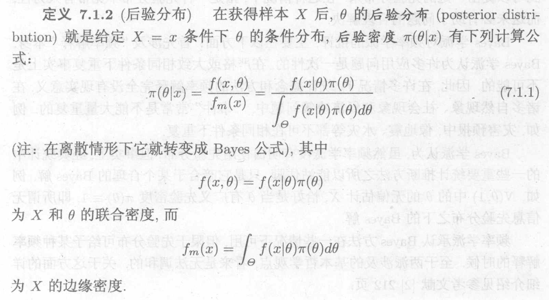
Def: posterior distribution
5.1. parameter estimate
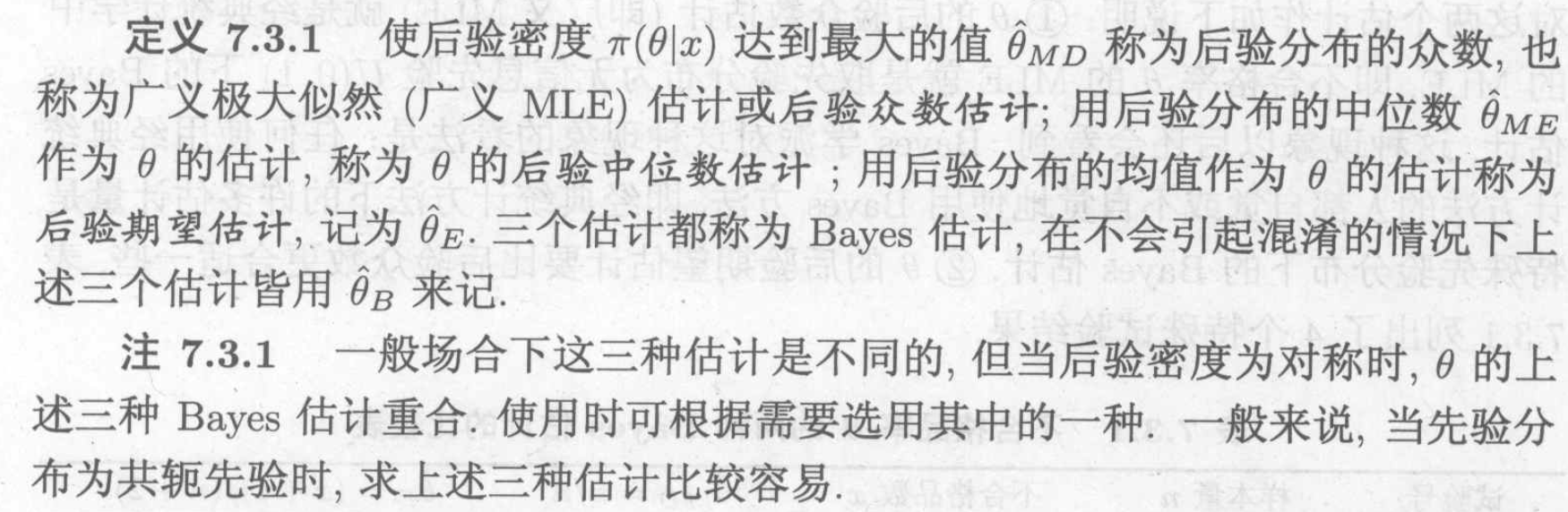
5.1.1. point estimate
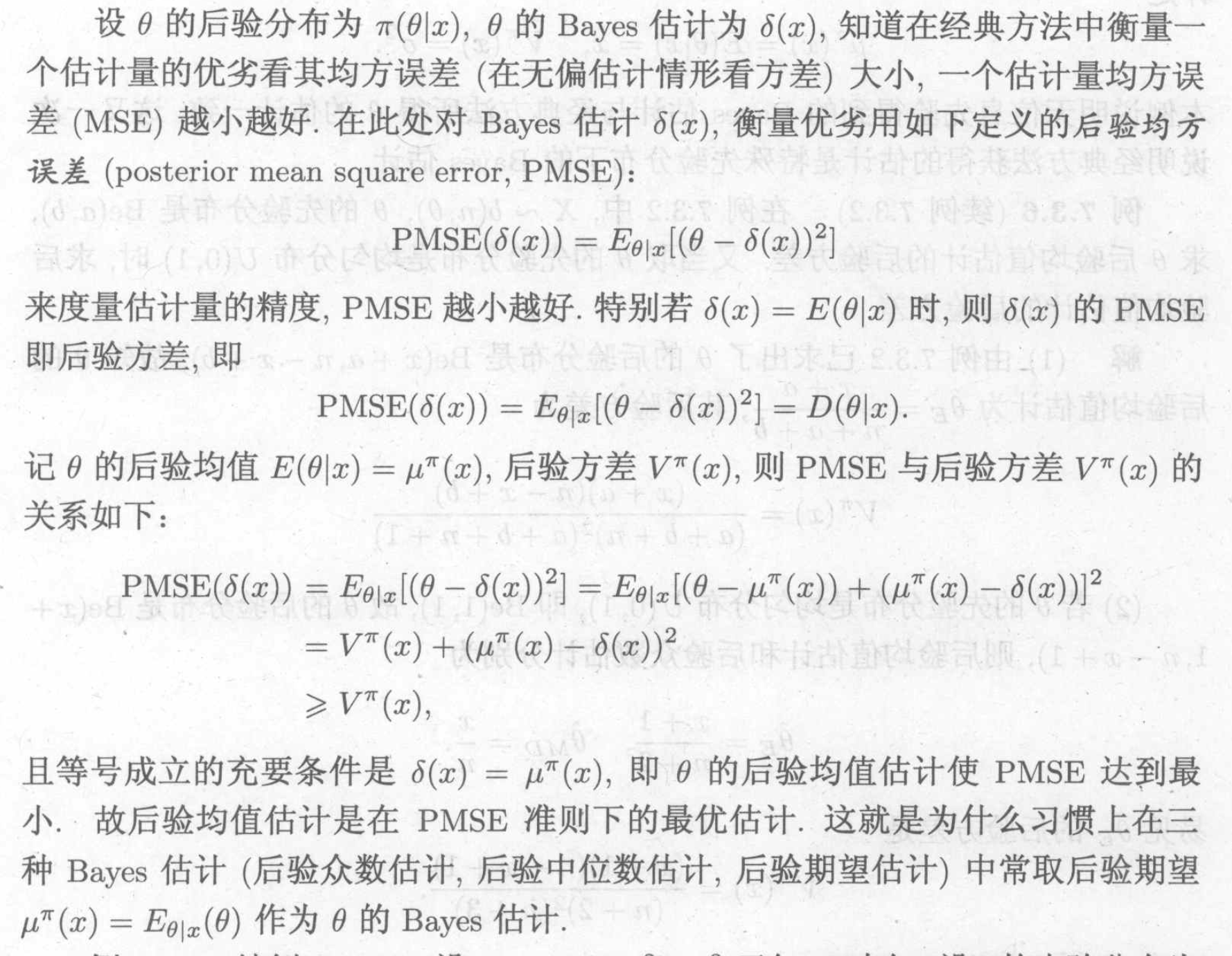
Def: bayes point estimate
Def: P-MSE
Usage: measurement of bayes point estimate
5.1.2. interval estimate
Def: bayers credible estimate
Note: difference between traditional
5.2. hypothesis test
Def: general methods
5.3. bayes decision theory
Def: decision problem
Def: decision rule
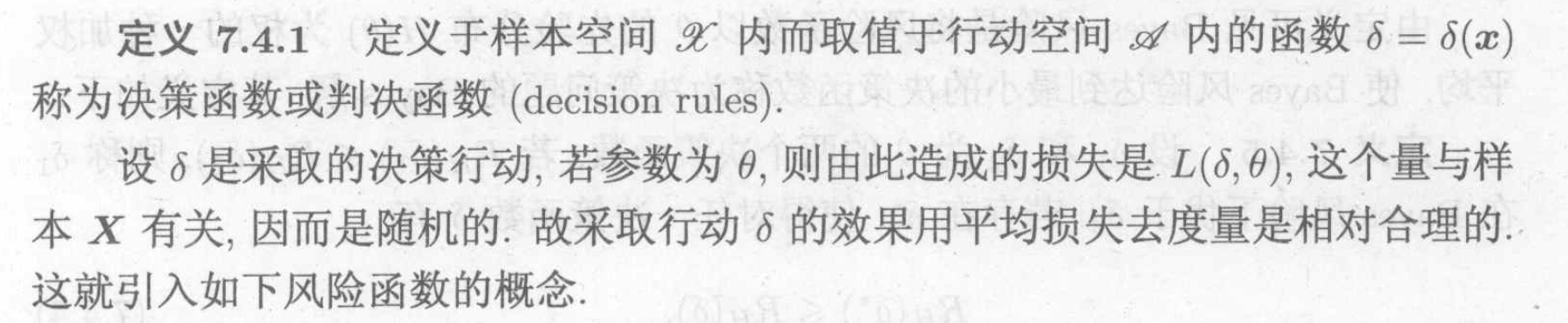
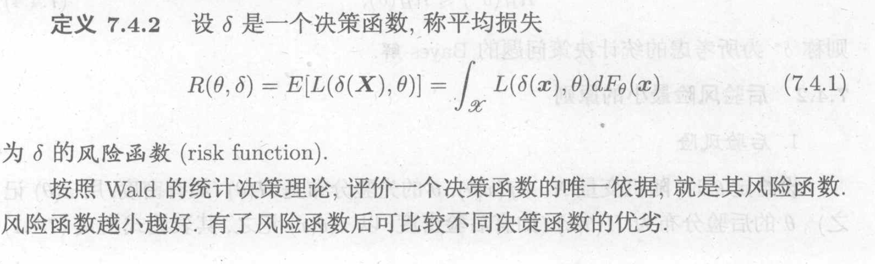
5.3.1. risk functions
Risk functions are basically different ways to get Expectation of loss function.
Def: risk function
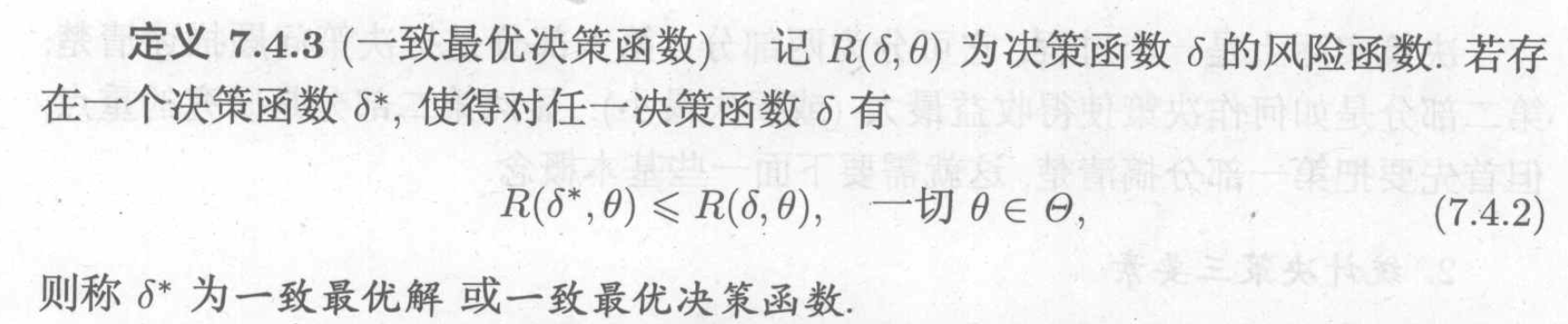
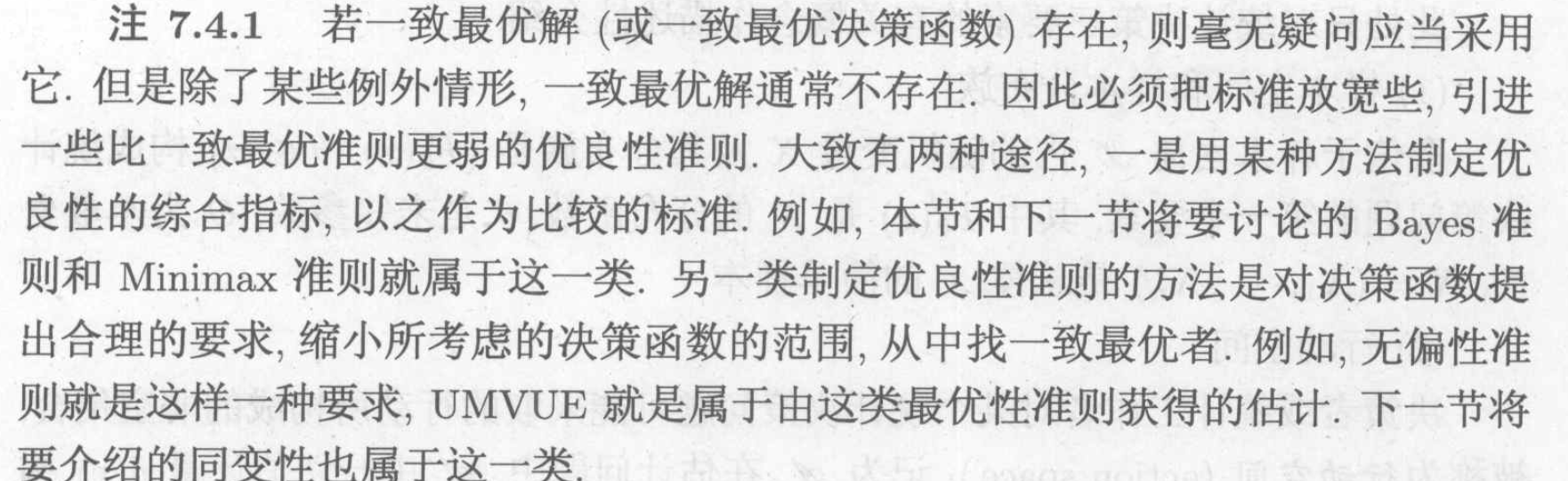
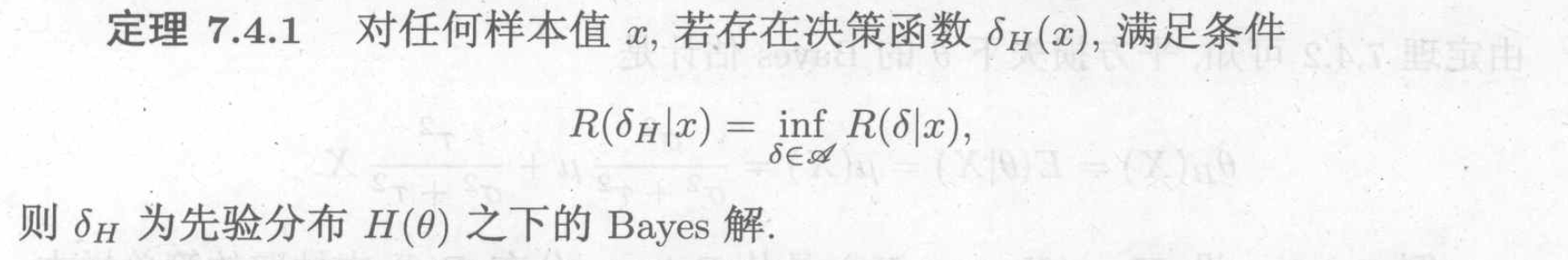
Def: optimal decision rule
Note:
Def: bayes risk function
Usage: since the general risk function do not always have optimal decision rule, we introduce bayes risk function
to conquer this issue .
Def: bayes optimal decision rule
Def: posterior risk
Note: relationship between posterior risk and bayes risk
Theorem: posterior risk & bayes risk yield the same thing .
5.3.2. loss functions
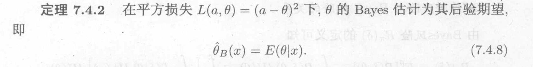
5.3.2.1. L2 loss
Theorem:
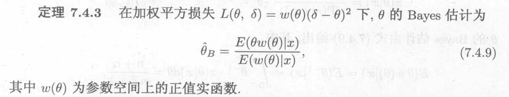
5.3.2.2. weighed L2 loss
Theorem:
5.3.2.3. L1 loss
Theorem:

6. sample space & stats
6.1. important stats
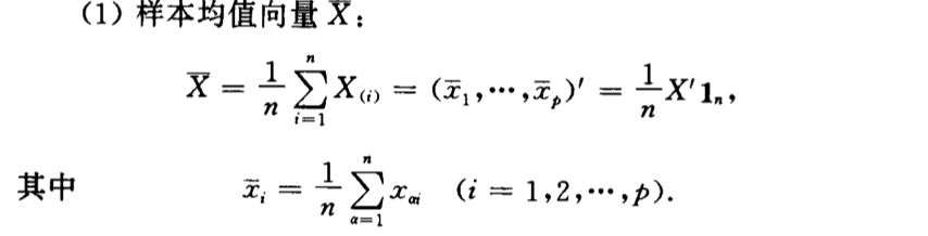
6.1.1. sample mean
Def: sample mean
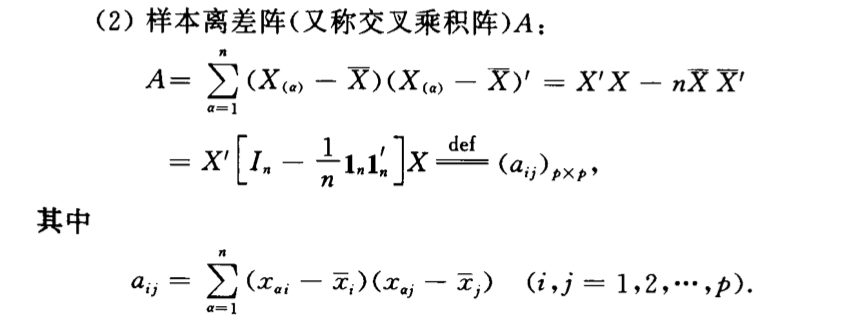
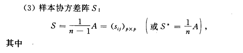
6.1.2. sample A
Def:
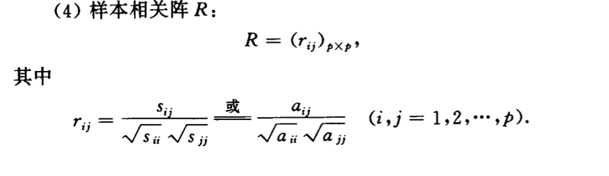
6.1.3. sample correlation
Def: sample correlation
6.1.4. sample coefficient
Def:
7. useful distributions
7.1. gaussian
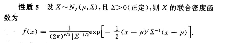
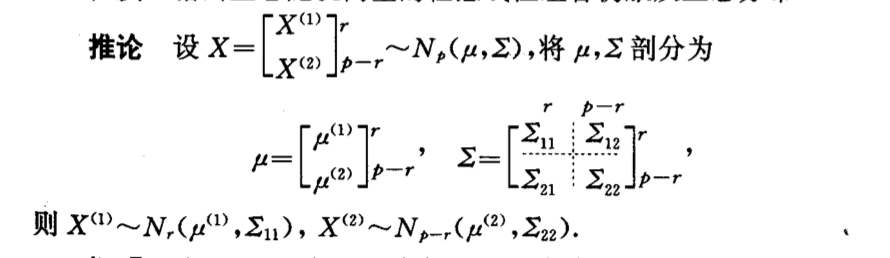
Def: multi-Gaussian
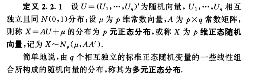
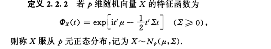
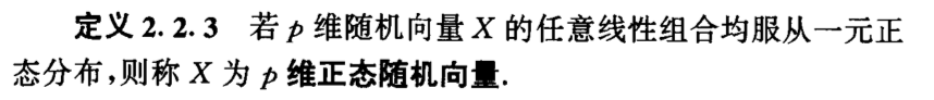
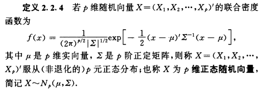
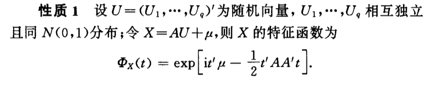
Qua: single =>

7.1.1. distribution
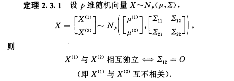
Def: distribution
Qua: operation

Qua: operation
7.1.1.1. transformation
Qua: 1
Qua: 2
Qua:
Qua:
Qua:
Qua:
Qua:

Qua:
Qua:
7.1.2. special function
Def: expectation

Def: charc
7.1.3. independence
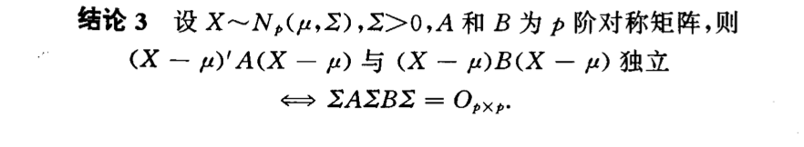
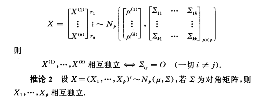
Theorem: of a vector
Corollary:

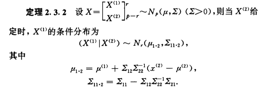
7.1.4. conditional
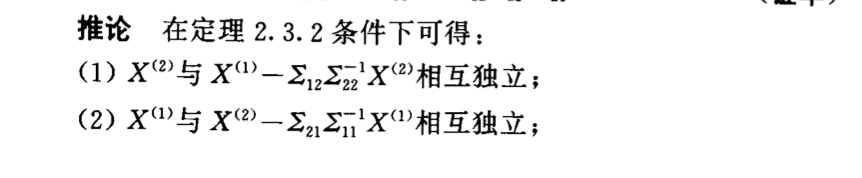
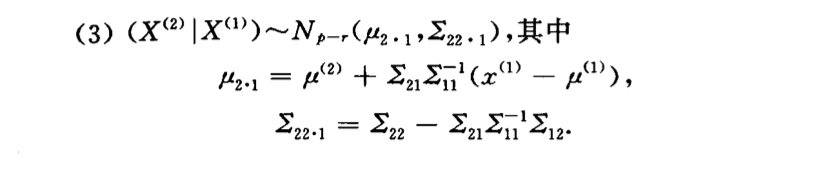
Def: conditional pdf
Corollary:
7.1.5. stats & estimations
7.1.5.1. stats
7.1.5.1.1. sample mean & variation
Theorem :
7.1.5.1.2. sample
7.1.5.2. estimations
Qua: =>
Theorem:
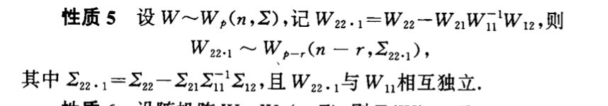
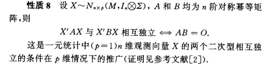
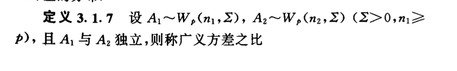
7.2. Wishart
Def:

7.2.1. distribution
7.2.1.1. tranformation
Qua:

Qua:
Qua:
Qua:
Qua:
Qua:
Qua:
7.2.2. special function
Def:

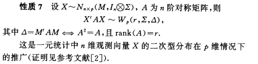
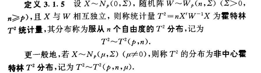
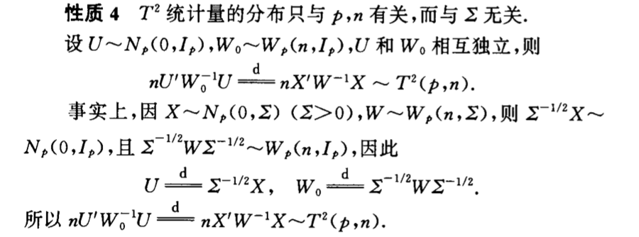
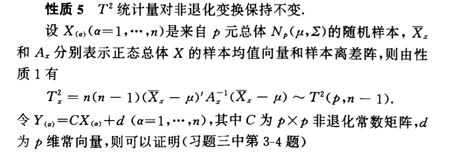
7.3. \(T^2\)
Def:
7.3.1. distribution
7.3.1.1. transformation
Qua:
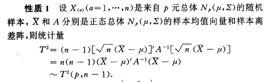
Qua:
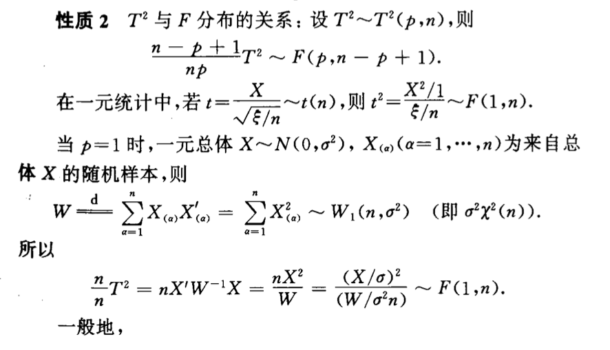
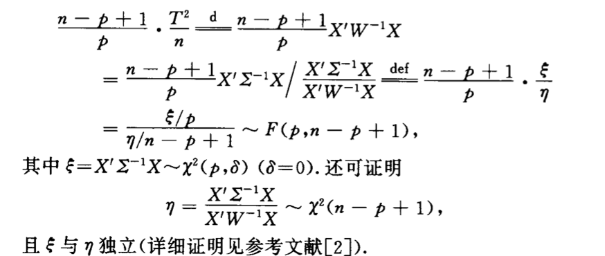
Qua:
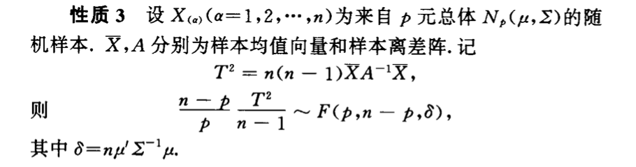
Qua:
Qua:
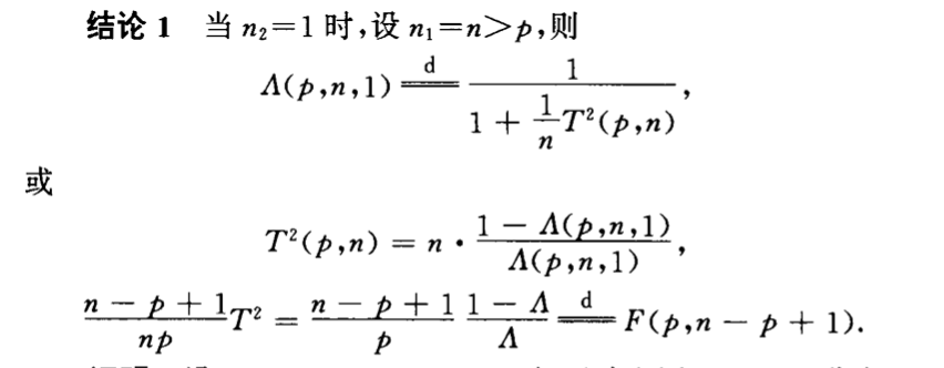
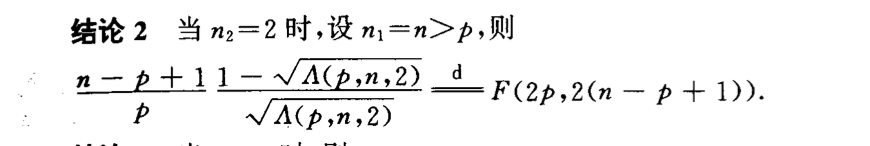
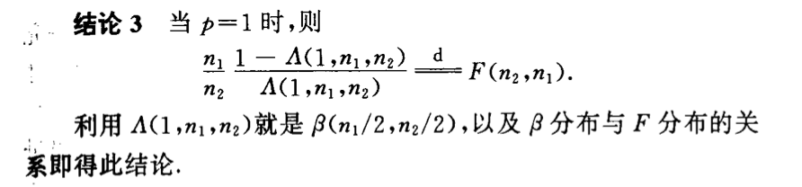
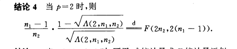
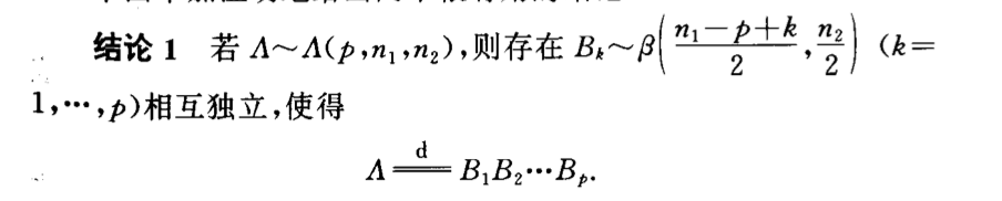
7.4. Wilks
Def:
7.4.1. distribution
7.4.1.1. tranformation
Qua:
Qua:
Qua:
Qua:
Qua:

Qua:
Qua:


8. parameter estimation
9. hypothesis test
P67